CCD calibration

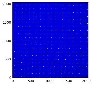
This tutorial presents how to calibrate the distortion from a CCD camera coupled with a taper of optic fibers. If your camera is already calibrated using Fit2D and you have access to the corresponding spline file, this tutorial is not for you: simply create your detector object like this pyFAI.detectors.Detector(splineFile="example.spline") and you are done. This tutorial uses the image of a regular grid on the detector.

It uses a procedure described in: “Calibration and correction of spatial distortions in 2D detector systems” from Hammersley, A. P.; Svensson, S. O.; Thompson, A. published in Nuclear Instruments and Methods in Physics Research Section A, Volume 346, Issue 1-2, p. 312-321. DOI:10.1016/0168-9002(94)90720-X

The procedure is performed in 4 steps:

1. peak picking
2. grid assignment
3. distortion fitting
4. interpolation of the fitted data
5. saving into a detector definition file

The picture used is the one of a regular metallic grid of holes (spaced by 5mm), just in front of the detector. We will assume holes are circular what looks correct in first approximation. Parallax error will be ignored in a first time.

Peak picking

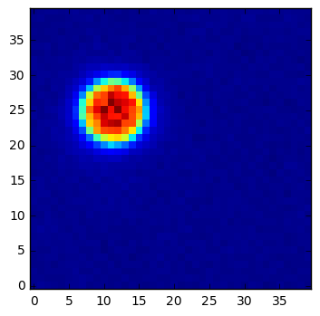
Lets start with peak picking, for this, we will use the FabIO library able to read the image and matplotlib to display the image. The distortion is assumed to be minimal in the middle of the detector, so we first focus on one spot in the middle:

#For final rendering switch from nbagg -> inline
#%pylab nbagg
%pylab inline

Populating the interactive namespace from numpy and matplotlib

# search for the image containing the grid
!ls *.edf

corrected.edf  frelonID22_grid.edf

fname = "frelonID22_grid.edf"
#fname = "corrected.edf"
import fabio
img = fabio.open(fname).data

WARNING:fabioimage:PIL is not installed ... trying to do without
WARNING:tifimage:PIL is not installed ... trying to do without
WARNING:bruker100image:PIL is not installed ... trying to do without
WARNING:xsdimage:lxml library is probably not part of your python installation: disabling xsdimage format

imshow(img, interpolation="nearest", origin="lower")

<matplotlib.image.AxesImage at 0x7f2c70f1add8>

#Zoom into a spot in the middle of the image, where the distortion is expected to be minimal
imshow(img[1060:1100,1040:1080], interpolation="nearest", origin="lower")

<matplotlib.image.AxesImage at 0x7f2c70ebbba8>

#Look at the profile of the peak to measure the width (it is expected to be a crenel)
plot(img[1060+25,1040:1060])

[<matplotlib.lines.Line2D at 0x7f2c70e383c8>]

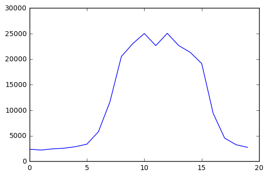
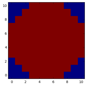
Let’s look at one spot, in the center of the image: it is circular and is slightly larger than 10 pixels. We will define a convolution kernel of size 11x11 of circular shape with sharp borders as this is what a perfect spot is expected to look like. The kernel is normalized in such a way it does not modify the average intensity of the image

Now convolve the image with this circular kernel using scipy.signal (in direct space: the kernel is small and performance does not really matter here).

It is important to have an odd size for the kernel for convolution as an even shape would induce an offset of 1/2 pixel in the located peak-position.

size = 11 #Odd of course
center = (size-1)//2
y, x = numpy.ogrid[-center:center+1,-center:center+1]
r2 = x*x + y*y
kernel = (r2<=(center+0.5)**2).astype(float)
kernel /= kernel.sum()
imshow(kernel, interpolation="nearest", origin="lower")

<matplotlib.image.AxesImage at 0x7f2c70d9c438>

from scipy import ndimage, signal

cnv = signal.convolve2d(img, kernel, mode="same")

#Check that size is unchanged.
print(img.shape)
print(cnv.shape)

(2048, 2048)
(2048, 2048)

#Check the image still looks the same. it is just supposed to be smoother.
imshow(cnv, origin="lower", interpolation="nearest")

<matplotlib.image.AxesImage at 0x7f2c5e259550>

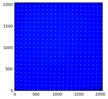
#Zoom into the very same spot to ensure it is smoother
imshow(cnv[1060:1100,1040:1080], interpolation="nearest", origin="lower")

<matplotlib.image.AxesImage at 0x7f2c5e1f8e80>

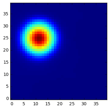
# and here again the same profile:
plot(cnv[1060+25,1030:1070])
# the peak got broader (2x) but much smoother on the top: this is what we are interrested in.

[<matplotlib.lines.Line2D at 0x7f2c5e160358>]

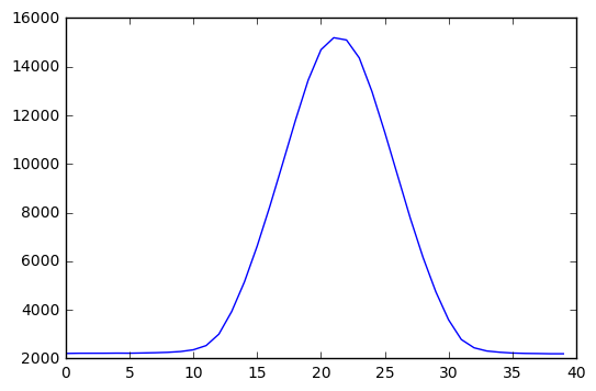
After convolution with a pattern of the same shape as the hole, the peak center is located with a sub-pixel resolution. The peak has a full size of 30 pixels in 1 dimension.

All peak positions will be extracted using the pyFAI inverse watershed algorithm. Once all regions are segmented, the ones too small are sieved out and the remaining ones are classifies according to their peak intensity using an histogram. As intensity vary a lot, this histogram it is done on the log-scale of the intensity.

mini = (kernel>0).sum()
print("Number of points in the kernel: %s"%mini)

Number of points in the kernel: 97

try: #depends if the version of pyFAI you are using
    from pyFAI.watershed import InverseWatershed
except:
    from pyFAI.ext.watershed import InverseWatershed
    #Version of pyFAI newer than feb 2016
iw = InverseWatershed(cnv)
iw.init()
iw.merge_singleton()
all_regions = set(iw.regions.values())
regions = [i for i in all_regions if i.size>mini]

print("Number of region segmented: %s"%len(all_regions))
print("Number of large enough regions : %s"%len(regions))

WARNING:pyFAI.utils:Exception No module named 'fftw3': FFTw3 not available. Falling back on Scipy
WARNING:pyFAI.opencl:Unable to import pyOpenCl. Please install it from: http://pypi.python.org/pypi/pyopencl
WARNING:pyFAI.timeit:init_labels took 1.104s
WARNING:pyFAI.timeit:init_borders took 0.048s
WARNING:pyFAI.timeit:init_regions took 0.450s
WARNING:pyFAI.timeit:init_pass took 0.143s
WARNING:pyFAI.timeit:merge_singleton took 0.033s

Number of region segmented: 79513
Number of large enough regions : 8443

s = [i.maxi for i in regions]
hist(numpy.log10(s), 20)
#Look for the maximum value in each region to be able to segment accordingly

(array([  1.00000000e+00,   0.00000000e+00,   0.00000000e+00,
          0.00000000e+00,   0.00000000e+00,   0.00000000e+00,
          0.00000000e+00,   0.00000000e+00,   0.00000000e+00,
          1.00000000e+00,   2.85000000e+02,   5.99900000e+03,
          1.71900000e+03,   1.00000000e+00,   0.00000000e+00,
          1.00000000e+00,   3.00000000e+00,   2.30000000e+01,
          1.17000000e+02,   2.93000000e+02]),
 array([ 2.05537045,  2.1621182 ,  2.26886594,  2.37561369,  2.48236143,
         2.58910918,  2.69585692,  2.80260467,  2.90935241,  3.01610016,
         3.1228479 ,  3.22959565,  3.33634339,  3.44309114,  3.54983888,
         3.65658663,  3.76333437,  3.87008212,  3.97682986,  4.08357761,
         4.19032535]),
 <a list of 20 Patch objects>)

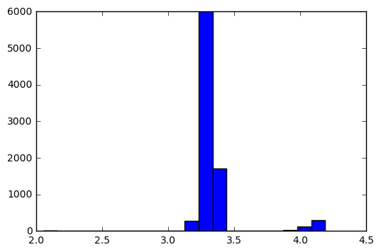
There are clearly 3 groups of very different intensity, well segregated:

• around (~125), those are the peaks where no tapper brings light
• around (~2500), those are segmented region in the background
• above (~8000), those are actual peaks, we are looking for.

We retain all peaks >

peaks = [(i.index//img.shape[-1], i.index%img.shape[-1]) for i in regions if (i.maxi)>10**3.5]
print("Number of remaining peaks: %s"%len(peaks))

Number of remaining peaks: 438

imshow(img, interpolation="nearest", origin="lower")
peaks_raw = numpy.array(peaks)
plot(peaks_raw[:,1], peaks_raw[:, 0], "or")
xlim(0,2048)
ylim(0,2048)
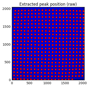
title("Extracted peak position (raw)")
print("Raw peak coordinate:")
print(peaks[:10])

Raw peak coordinate:
[(1273, 2027), (1664, 1742), (1666, 1646), (1866, 1155), (1274, 1933), (1867, 466), (1867, 563), (1867, 1056), (203, 1131), (107, 1226)]

Precise peak extraction is performed using a second order tailor expansion

try:
    from pyFAI.bilinear import Bilinear
except:
    from pyFAI.ext.bilinear import Bilinear
bl = Bilinear(cnv)

ref_peaks = [bl.local_maxi(p) for p in peaks]
imshow(img, interpolation="nearest", origin="lower")
peaks_ref = numpy.array(ref_peaks)
plot(peaks_raw[:,1], peaks_raw[:, 0], "or")
plot(peaks_ref[:,1],peaks_ref[:, 0], "ob")
xlim(0,2048)
ylim(0,2048)
title("Extracted peak position (red: raw, blue: refined)")
print("Refined peak coordinate:")
print(ref_peaks[:10])

Refined peak coordinate:
[(1272.9463423714042, 2026.5502902269363), (1664.0545781441033, 1742.1054049506783), (1666.296777099371, 1645.9045108556747), (1866.365830898285, 1154.7454472184181), (1274.126026943326, 1932.9975793703925), (1866.5777518451214, 465.5264100730419), (1867.4438569247723, 563.2241970151663), (1867.3492084741592, 1056.0545778758824), (203.06922163814306, 1131.10803706944), (106.92814844101667, 1226.3799100518227)]

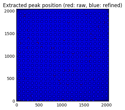
At this stage, a visual inspection of the grid confirms all peaks have been properly segmented. If this is not the case, one can adapt:

• the size of the kernel
• the threshold coming out of the histogramming

Pair-wise distribution function

We will now select the (4-) first neighbours for every single peak. For this we calculate the distance_matrix from any point to any other:

# Nota, pyFAI uses **C-coordinates** so they come out as (y,x) and not the usual (x,y).
# This notation helps us to remind the order
yx = numpy.array(ref_peaks)

# pairwise distance calculation using scipy.spatial.distance_matrix
from scipy.spatial import distance_matrix
dist = distance_matrix(peaks_ref, peaks_ref)

Let’s have a look at the pairwise distribution function for the first neighbors

hist(dist.ravel(), 200, range=(0,200))
title("Pair-wise distribution function")

<matplotlib.text.Text at 0x7f2c4e3468d0>

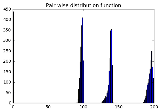
This histogram provides us:

• At 0, the 438 peaks with 0-distance to themselves.
• between 85 and 105 the first neighbours
• between 125 and 150 the second neighbours.
• ... and so on.

We now focus on the first neighbours which are all located between 70 and 110 pixels apart.

#We define here a data-type for each peak (called center) with 4 neighbours (called north, east, south and west).
point_type = np.dtype([('center_y', float), ('center_x', float),
                        ('east_y', float), ('east_x', float),
                        ('west_y', float), ('west_x', float),
                        ('north_y', float), ('north_x', float),
                        ('south_y', float), ('south_x', float)])

neig = np.logical_and(dist>70.0, dist<110.0)
valid = (neig.sum(axis=-1)==4).sum()
print("There are %i control point with exactly 4 first neigbours"%valid)
# This initializes an empty structure to be populated
point = numpy.zeros(valid, point_type)

There are 359 control point with exactly 4 first neigbours

#Populate the structure: we use a loop as it loops only over 400 points
h=-1
for i, center in enumerate(peaks_ref):
    if neig[i].sum()!=4: continue
    h+=1
    point[h]["center_y"],point[h]["center_x"] = center
    for j in ((0,1),(0,-1),(1,0),(-1,0)):
        tmp = []
        for k in numpy.where(neig[i]):
            curr = yx[k]
            tmp.append(dot(curr-center,j))
            l = argmax(tmp)
            y, x = peaks_ref[numpy.where(neig[i])][l]
            if j==(0,1):point[h]["east_y"], point[h]["east_x"] = y, x
            elif j==(0,-1):point[h]["west_y"], point[h]["west_x"] = y, x
            elif j==(1,0): point[h]["north_y"],point[h]["north_x"] = y, x
            elif j==(-1,0):point[h]["south_y"],point[h]["south_x"] = y, x

We will need to define an origin but taking it on the border of the image is looking for trouble as this is where distortions are likely to be the most important. The center of the detector is an option but we prefer to take the peak the nearest to the centroid of all other peaks.

#Select the initial guess for the center:

#Most intense peak:
#m = max([i for i in regions], key=lambda i:i.maxi)
#Cx, Cy = m.index%img.shape[-1],m.index//img.shape[-1]
#Cx, Cy = point["center_x"].mean(), point["center_y"].mean() #Centroid of all points
Cx, Cy = 734, 1181 #beam center
#Cx, Cy = tuple(i//2 for i in cnv.shape) #detector center
print("The guessed center is at (%s, %s)"%(Cx, Cy))

#Get the nearest point from centroid:
d2 = ((point["center_x"]-Cx)**2+(point["center_y"]-Cy)**2)
best = d2.argmin()
Op = point[best]
Ox, Oy = Op["center_x"], Op["center_y"]

print("The center is at (%s, %s)"%(Ox, Oy))
#Calculate the average vector along the 4 main axes
Xx = (point[:]["east_x"] - point[:]["center_x"]).mean()
Xy = (point[:]["east_y"] - point[:]["center_y"]).mean()
Yx = (point[:]["north_x"] - point[:]["center_x"]).mean()
Yy = (point[:]["north_y"] - point[:]["center_y"]).mean()

print("The X vector is is at (%s, %s)"%(Xx, Xy))
print("The Y vector is is at (%s, %s)"%(Yx, Yy))

The guessed center is at (734, 1181)
The center is at (753.703500152, 1186.18798503)
The X vector is is at (97.7197301826, -0.787977117653)
The Y vector is is at (1.38218579497, 97.0826990758)

print("X has an angle of %s deg"%rad2deg(arctan2(Xy, Xx)))
print("Y has an angle of %s deg"%rad2deg(arctan2(Yy, Yx)))
print("The XY angle is %s deg"%rad2deg(arctan2(Yy, Yx)-arctan2(Xy, Xx)))

X has an angle of -0.462002756355 deg
Y has an angle of 89.1843236418 deg
The XY angle is 89.6463263982 deg

x = point[:]["center_x"] - Ox
y = point[:]["center_y"] - Oy
xy = numpy.vstack((x,y))
R = numpy.array([[Xx,Yx],[Xy,Yy]])
iR = numpy.linalg.inv(R)
IJ = dot(iR,xy).T

Xmin = IJ[:,0].min()
Xmax = IJ[:,0].max()
Ymin = IJ[:,1].min()
Ymax = IJ[:,1].max()
print("Xmin/max", Xmin, Xmax)
print("Ymin/max", Ymin, Ymax)
print("Maximum error versus integrer: %s * pitch size (5mm)"%(abs(IJ-IJ.round()).max()))

Xmin/max -6.07394212848 12.060721056
Ymin/max -11.0890545732 7.04060363671
Maximum error versus integrer: 0.117211354675 * pitch size (5mm)

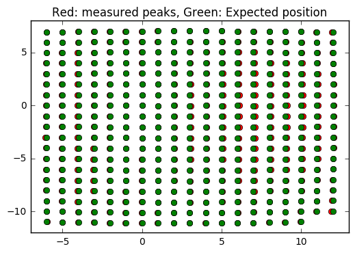
At this point it is important to check the correct rounding to integers: The maximum error should definitely be better than 0.2*pitch ! If not, try to change the origin (Cx and Cy). This criteria will be used for the optimization later on.

plot(IJ[:,0],IJ[:,1],"or")
idx = numpy.round(IJ).astype(int)
plot(idx[:,0],IJ[:,1],"og")
xlim(floor(Xmin), ceil(Xmax))
ylim(floor(Ymin), ceil(Ymax))
title("Red: measured peaks, Green: Expected position")

<matplotlib.text.Text at 0x7f2c4e313278>

Estimation of the pixel size:

The pixel size is obtained from the pitch of the grid, in vectorial:

pitch = 5e-3 #mm distance between holes
Py = pitch*sqrt((Yx**2-Xx**2)/((Xy*Yx)**2-(Xx*Yy)**2))
Px = sqrt((pitch**2-(Xy*Py)**2)/Xx**2)
print("Pixel size in average: x:%.3f micron, y: %.3f microns"%(Px*1e6, Py*1e6))

Pixel size in average: x:51.165 micron, y: 51.497 microns

At this stage, we have:

• A list of control points placed on a regular grid with a sub-pixel precision
• The center of the image, located on a control point
• the average X and Y vector to go from one control point to another

Optimization of the pixel position

The optimization is obtained by minimizing the mis-placement of the control points on the regular grid. For a larger coverage we include now the peaks on the border with less than 4 neighbours.

#Measured peaks (all!), needs to flip x<->y
peaks_m = numpy.empty_like(peaks_ref)
peaks_m[:,1] = peaks_ref[:,0]
peaks_m[:,0] = peaks_ref[:,1]

#parameter set for optimization:
P0 = [Ox, Oy, Xx, Yx, Xy, Yy]

P = numpy.array(P0)

def to_hole(P, pixels):
    "Translate pixel -> hole"
    T = numpy.atleast_2d(P[:2])
    R = P[2:].reshape((2,2))
    #Transformation matrix from pixel to holes:
    hole = dot(numpy.linalg.inv(R), (pixels - T).T).T
    return hole

def to_pix(P, holes):
    "Translate hole -> pixel"
    T = numpy.atleast_2d(P[:2])
    R = P[2:].reshape((2,2))
    #Transformation from index points (holes) to pixel coordinates:
    pix = dot(R,holes.T).T + T
    return pix

def error(P):
    "Error function"
    hole_float = to_hole(P, peaks_m)
    hole_int = hole_float.round()
    delta = hole_float-hole_int
    delta2 = (delta**2).sum()
    return delta2

print("Total inital error ", error(P), P0)
holes = to_hole(P, peaks_m)
print("Maximum initial error versus integrer: %s * pitch size (5mm)"%(abs(holes-holes.round()).max()))
from scipy.optimize import minimize
res = minimize(error, P)
print(res)
print("total Final error ", error(res.x),res.x)
holes = to_hole(res.x, peaks_m)
print("Maximum final error versus integrer: %s * pitch size (5mm)"%(abs(holes-holes.round()).max()))

Total inital error  2.5995763607 [753.70350015163422, 1186.1879850327969, 97.719730182623479, 1.3821857949656571, -0.78797711765336542, 97.082699075794565]
Maximum initial error versus integrer: 0.199838456433 * pitch size (5mm)
      fun: 2.123772842169884
 hess_inv: array([[  1.41698853e+01,   5.02981780e-01,  -8.67450996e-01,
          5.65400698e-01,  -2.23588556e-02,   3.62469793e-02],
       [  5.02981780e-01,   1.44432486e+01,  -6.17043562e-03,
          3.18737250e-02,  -8.80159842e-01,   5.53478243e-01],
       [ -8.67450996e-01,  -6.17043562e-03,   2.99705132e-01,
         -4.12312169e-03,   2.39113093e-03,  -1.79968692e-03],
       [  5.65400698e-01,   3.18737250e-02,  -4.12312169e-03,
          3.01702833e-01,  -1.78715958e-03,   3.83867286e-03],
       [ -2.23588556e-02,  -8.80159842e-01,   2.39113093e-03,
         -1.78715958e-03,   2.97818929e-01,  -3.46536500e-03],
       [  3.62469793e-02,   5.53478243e-01,  -1.79968692e-03,
          3.83867286e-03,  -3.46536500e-03,   2.93190623e-01]])
      jac: array([ -2.98023224e-08,   5.66244125e-07,   1.19209290e-07,
         3.57627869e-07,   8.34465027e-07,   1.10268593e-06])
  message: 'Optimization terminated successfully.'
     nfev: 160
      nit: 15
     njev: 20
   status: 0
  success: True
        x: array([  7.53021133e+02,   1.18519693e+03,   9.81143528e+01,
         1.47509462e+00,  -8.04478941e-01,   9.73166902e+01])
total Final error  2.12377284217 [  7.53021133e+02   1.18519693e+03   9.81143528e+01   1.47509462e+00
  -8.04478941e-01   9.73166902e+01]
Maximum final error versus integrer: 0.234645015537 * pitch size (5mm)

clf()
peaks_c = to_pix(res.x,to_hole(res.x,peaks_m).round())
imshow(img, interpolation="nearest", origin="lower")
plot(peaks_m[:,0],peaks_m[:, 1], "or")
plot(peaks_c[:,0], peaks_c[:, 1], "og")
xlim(0,2048)
ylim(0,2048)
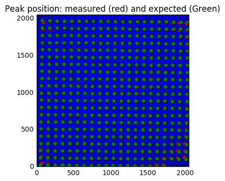
title("Peak position: measured (red) and expected (Green)")

<matplotlib.text.Text at 0x7f2c4e3de668>

pitch = 5e-3 #mm distance between holes
Ox, Oy, Xx, Yx, Xy, Yy = res.x
Py = pitch*sqrt((Yx**2-Xx**2)/((Xy*Yx)**2-(Xx*Yy)**2))
Px = sqrt((pitch**2-(Xy*Py)**2)/Xx**2)
print("Optimized pixel size in average: x:%.3f micron, y: %.3f microns"%(Px*1e6, Py*1e6))

Optimized pixel size in average: x:50.959 micron, y: 51.373 microns

Few comments:

• The maximum error grow during optimization without explanations
• The outer part of the detector is the most distorted

Interpolation of the fitted data

Multivariate data interpolation (griddata)

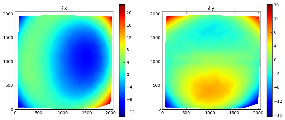
Correction arrays are built slightly larger (+1) to be able to manipulate corners instead of centers of pixels As coordinates are needed as y,x (and not x,y) we use p instead of peaks_m

from scipy.interpolate import griddata
grid_x, grid_y = np.mgrid[0:img.shape[0]+1, 0:img.shape[1]+1]
delta = peaks_c - peaks_m
#we use peaks_res instead of peaks_m to be in y,x coordinates, not x,y
delta_x = griddata(peaks_ref, delta[:,0], (grid_x, grid_y), method='cubic')
delta_y = griddata(peaks_ref, delta[:,1], (grid_x, grid_y), method='cubic')

figure(figsize=(12,5))
subplot(1,2,1)
imshow(delta_x,origin="lower", interpolation="nearest")
title(r"$\delta$ x")
colorbar()
subplot(1,2,2)
imshow(delta_y, origin="lower", interpolation="nearest")
title(r"$\delta$ y")
colorbar()
#Nota: the arrays are filled with "NaN" outside the convex Hull

<matplotlib.colorbar.Colorbar at 0x7f2c47ed3d30>

#From http://stackoverflow.com/questions/3662361/fill-in-missing-values-with-nearest-neighbour-in-python-numpy-masked-arrays
def fill(data, invalid=None):
    """
    Replace the value of invalid 'data' cells (indicated by 'invalid')
    by the value of the nearest valid data cell

    Input:
        data:    numpy array of any dimension
        invalid: a binary array of same shape as 'data'. True cells set where data
                 value should be replaced.
                 If None (default), use: invalid  = np.isnan(data)

    Output:
        Return a filled array.
    """

    if invalid is None:
        invalid = numpy.isnan(data)

    ind = ndimage.distance_transform_edt(invalid, return_distances=False, return_indices=True)
    return data[tuple(ind)]

figure(figsize=(12,5))
subplot(1,2,1)
imshow(fill(delta_x),origin="lower", interpolation="nearest")
title(r"$\delta$ x")
colorbar()
subplot(1,2,2)
imshow(fill(delta_y), origin="lower", interpolation="nearest")
title(r"$\delta$ y")
colorbar()

<matplotlib.colorbar.Colorbar at 0x7f2c46c55f98>

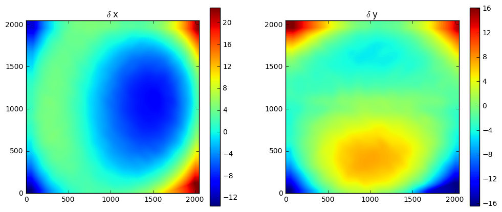
It is important to understand the extrapolation outside the convex hull has no justification, it is there just to prevent numerical bugs.

Saving the distortion correction arrays to a detector

from pyFAI.detectors import Detector
detector = Detector(Py,Px)
detector.max_shape = detector.shape = img.shape
detector.set_dx(fill(delta_x))
detector.set_dy(fill(delta_y))
detector.mask = numpy.isnan(delta_x).astype(numpy.int8)[:img.shape[0], :img.shape[1]]
detector.save("testdetector.h5")

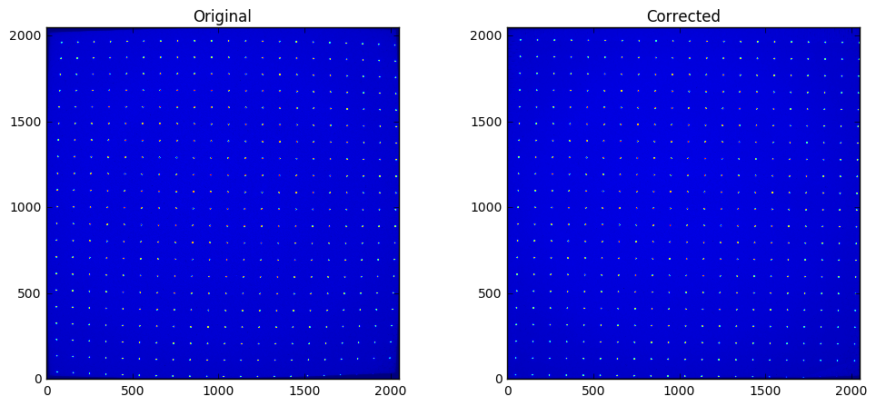
Validation of the distortion correction

from pyFAI.distortion import Distortion
dis = Distortion(detector)
cor = dis.correct(img)
figure(figsize=(12,5))
subplot(1,2,1)
imshow(img, interpolation="nearest", origin="lower")
title("Original")
subplot(1,2,2)
imshow(cor, origin="lower", interpolation="nearest")
title("Corrected")
fabio.edfimage.EdfImage(data=cor).save("corrected.edf")

Conclusion

This procedure describes how to measure the detector distortion and how to create a detector description file directly usable in pyFAI. Only the region inside the convex hull of the grid data-points is valid and the region of the detector which is not calibrated has been masked out to prevent accidental use of it.

The distortion corrected image can now be used to check how “good” the calibration actually is. This file can be injected in the third cell, and follow the same procedure (left as exercise). This gives a maximum mis-placement of 0.003, the average error is then of 0.0006 and correction-map exhibit a displacement of pixels in the range +/- 0.2 pixels which is acceptable and validates the whole procedure.