General introduction
Python Fast Azimuthal Integration
PyFAI is implemented in Python programming language, which is open source and already very popular for scientific data analysis ([PyMca], [PyNX], …). It relies on the scientific stack of python composed of [NumPy], [SciPy] and [Matplotlib] plus the [OpenCL] binding [PyOpenCL] for performances.
\(2D\) area detectors like CCD or pixel detectors have become popular in the last 15 years for diffraction experiments (e.g. for WAXS, SAXS, single crystal and powder diffraction). These detectors have a large sensitive area of millions of pixels with high spatial resolution. The software package pyFAI ([SRI2012], [EPDIC13]) has been designed to reduce SAXS, WAXS and XRPD images taken with those detectors into \(1D\) curves (azimuthal integration) usable by other software for in-depth analysis such as Rietveld refinement, or \(2D\) images (a radial transformation named caking in [FIT2D]). As a library, the aim of pyFAI is to be integrated into other tools like [PyMca] or [EDNA] or [LImA] with a clean pythonic interface. However pyFAI features also command line and graphical tools for batch processing, converting data into q-space (q being the momentum transfer) or 2\(\theta\)-space (\(\theta\) being the Bragg angle) and a calibration graphical interface for optimizing the geometry of the experiment using the Debye-Scherrer rings of a reference sample. PyFAI shares the geometry definition of SPD but can directly import geometries determined by the software FIT2D. PyFAI has been designed to work with any kind of detector and geometry (transmission or reflection) and relies on FabIO, a library able to read more than 20 image formats produced by detectors from 12 different manufacturers. During the transformation from cartesian space \((x,y)\) to polar space \((2\theta, \chi )\), both local and total intensities are conserved in order to obtain accurate quantitative results. Technical details on how this integration is implemented and how it has been ported to native code and parallelized on graphic cards are quickly presented but you can refer to this publications for further details.
Introduction
With the advent of hyperspectral experiments like diffraction tomography in the world of synchrotron radiation, existing software tools for azimuthal integration like [FIT2D] and [SPD] reached their performance limits owing to the fast data rate needed by such experiments. Even when integrated into massively parallel frameworks like [EDNA] , such stand-alone programs, due to their monolithic nature, cannot keep the pace with the data flow of new detectors. Therefore we decided to implemente from scratch a novel azimuthal integration tool which is designed to take advantage of modern parallel hardware features. PyFAI assumes the setup does not change during the experiment and tries to reuse a maximum number of data (using memoization), moreover those calculation are performed only when needed (lazy evaluation).
Experiment description
In pyFAI, the basic experiment is defined by a description of an area-detector whose position in space is defined through the sample position and the incident X-ray beam, and can be calibrated using Debye-Scherrer rings of a reference compound.
Geometry
Geometry conversion
Calibration
PyFAI executables
PyFAI was designed to be used by scientists needing a simple and effective tool for azimuthal integration. There are a certain number of scripts which will help you in preprocessing images (dark current, flat-field, averaging, …), calibrating the geometry, performing the integration. Finally couple of specialized tool called diff_tomo and diff_map are available to reduce a 2D/3D-mapping experiment of 2D images into a 3D volume (\(x, y, 2\theta\) for mapping or \(rot, trans, 2\theta\) for tomography)
There are cookbooks on these scripts in Cookbook recipes and their complete manual pages are available in the Application manuals section.
Python library
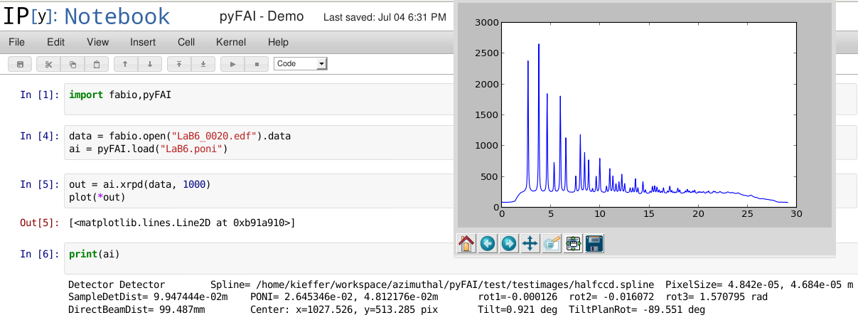
PyFAI is first and foremost a library: a tool of the scientific toolbox built around [IPython] and [NumPy] to perform data analysis either interactively or via scripts. Figure [notebook] shows an interactive session where an integrator is created, and an image loaded and integrated before being plotted.

The tutorial section makes heavy use of Jupyter notebooks to process data using pyFAI. The first tutorial also explains a bit how Python and Jupyter works to be able to perform basic processing efficiently with pyFAI.
Regrouping mechanism
In pyFAI, regrouping is performed using a histogram-like algorithm. Each pixel of the image is associated to its polar coordinates \((2\theta , \chi )\) or \((q, \chi )\), then a pair of histograms versus \(2\theta\) (or \(q\)) are built, one non weighted for measuring the number of pixels falling in each bin and another weighted by pixel intensities (after dark-current subtraction, and corrections for flat-field, solid-angle and polarization). The division of the weighted histogram by the number of pixels per bin gives the average signal over the given corona which provides the diffraction pattern. \(2D\) regrouping (called caking in FIT2D) is obtained in the same way using two-dimensional histograms over radial (\(2\theta\) or \(q\)) and azimuthal angles (\(\chi\)).
Pixel splitting algorithm
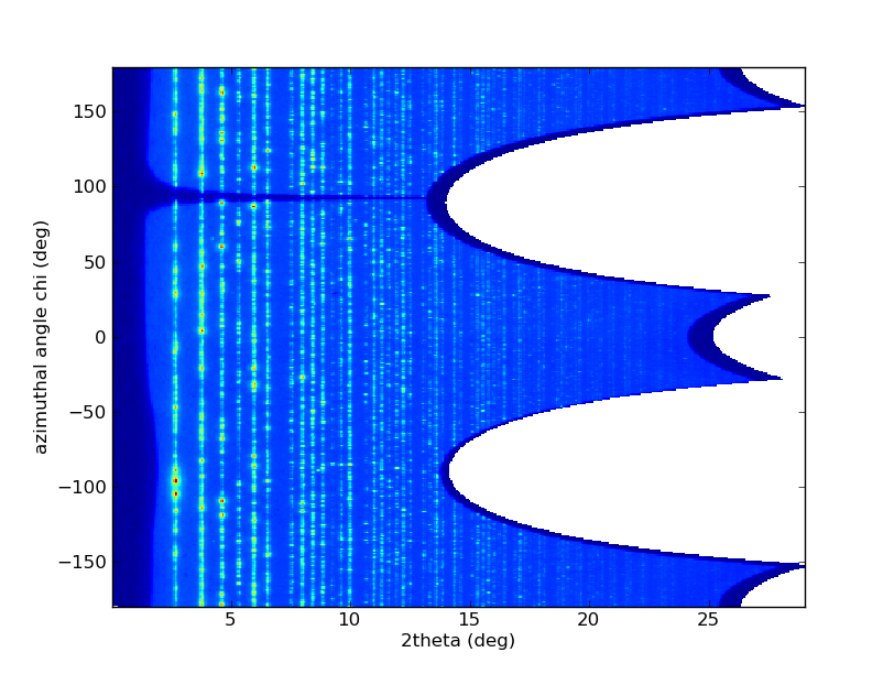
Powder diffraction patterns obtained by histogramming have a major weakness where pixel statistics are low. A manifestation of this weakness becomes apparent in the \(2D\)-regrouping where most of the bins close to the beam-stop are not populated by any pixel. In this figure, many pixels are missing in the low \(2\theta\) region, due to the arbitrary discretization of the space in pixels as intensities were assigned to each pixel center which does not reflect the physical reality of the scattering experiment.

PyFAI solves this problem by pixel splitting : in addition to the pixel position, its spatial extension is calculated and each pixel is then split and distributed over the corresponding bins, the intensity being considered as homogeneous within a pixel and spread accordingly. The drawback of this is the correlation introduced between two adjacent bins. To simplify calculations, this was initially done by abstracting the pixel shape with a bounding box that circumscribes the pixel. In an effort to better the quality of the results this method was dropped in favoor of a full pixel splitting scheme that actually uses the actual pixel geometry for its calculations.

Performances and migration to native code
Originally, regrouping was implemented using the histogram provided by [NumPy], then re-implemented in [Cython] with pixel splitting to achieve a four-fold speed-up. The computation time scales like O(N) with the size of the input image. The number of output bins shows only little influence; overall the single threaded [Cython] implementation has been stated at 30 Mpix/s (on a 3.4 GHz Intel core i7-2600).
Parallel implementation
The method based on histograms works well on a single processor but runs into problems requiring so called “atomic operations” when run in parallel. Processing pixels in the input data order causes write access conflicts which become less efficient with the increase of number of computing units (need of atomic_operation). This is the main limit of the method exposed previously; especially on GPU where thousands of threads are executed simultaneously.
To overcome this limitation; instead of looking at where input pixels GO TO in the output image, we instead look at where the output pixels COME FROM in the input image. This transformation is called a “scatter to gather” transformation in parallel programming.
The correspondence between pixels and output bins can be stored in a look-up table (LUT) together with the pixel weight which make the integration look like a simple (if large and sparse) matrix vector product. This look-up table size depends on whether pixels are split over multiple bins and to exploit the sparse structure, both index and weight of the pixel have to be stored. We measured that 500 Mbytes are needed to store the LUT to integrate a 16 megapixels image, which fits onto a reasonable quality graphics card nowadays but can still be too large to fit on an entry-level graphics card.
By making this change we switched from a “linear read / random write” forward algorithm to a “random read / linear write” backward algorithm which is more suitable for parallelization. As a farther improvement on the algorithm, the use of compressed sparse row (CSR) format was introduced, to store the LUT data. This algorithm was implemented both in [Cython]-OpenMP and OpenCL. The CSR approach has a double benefit: first, it reduces the size of the storage needed compared to the LUT by a factor two to three, offering the opportunity of working with larger images on the same hardware. Secondly, the CSR implementation in OpenCL is using an algorithm based on multiple parallel reductions where many execution threads are collaborating to calculate the content of a single bin. This makes it very well suited to run on GPUs and accelerators where hundreds to thousands of simultaneous threads are available.
When using OpenCL for the GPU we used a compensated (or Kahan_summation), to reduce the error accumulation in the histogram summation (at the cost of more operations to be done). This allows accurate results to be obtained on cheap hardware that performs calculations in single precision floating-point arithmetic (32 bits) which are available on consumer grade graphic cards. Double precision operations are currently limited to high price and performance computing dedicated GPUs. The additional cost of Kahan summation, 4x more arithmetic operations, is hidden by smaller data types, the higher number of single precision units and that the GPU is usually limited by the memory bandwidth anyway.
Conclusion
The library pyFAI was developed with two main goals:
- Performing azimuthal integration with a clean programming interface.
- No compromise on the quality of the results is accepted: a careful management of the geometry and precise pixel splitting ensures total and local intensity preservation.
PyFAI is the first implementation of an azimuthal integration algorithm on a GPUs as far as we are aware of, and the stated twenty-fold speed up opens the door to a new kind of analysis, not even considered before. With a good interface close to the camera, we believe PyFAI is able to sustain the data streams from the next generation high-speed detectors.
Acknowledgments
Porting pyFAI to GPU would have not been possible without the financial support of LinkSCEEM-2 (RI-261600).