Representation of a Fiber Diffraction / Grazing Incidence pattern
As with fibers, during a grazing-incidence scattering experiments (GIWAXS, GISAXS) on a thin film, a fiber symmetry is usually considered
Inside a fiber, there is a vertical axis with specific crystalline planes while the radial axis are equivalent
The same way, for a thin film, it is common to split the q vector in a vertical component (along the thickness axis) and an in-plane component
[1]:
from pyFAI.calibrant import get_calibrant
from pyFAI.detectors import RayonixLx255, Pilatus1M
from pyFAI.azimuthalIntegrator import AzimuthalIntegrator
from pyFAI.gui import jupyter
from pyFAI.test.utilstest import UtilsTest
from pyFAI.units import get_unit_fiber
import fabio
import numpy as np
from PIL import Image
from pyFAI import load
import matplotlib.pyplot as plt
import time
t0 = time.perf_counter()
In pyFAI:
x is the horizontal axis of the lab
y is the vertical axis of the lab
z is the beam propagation axis
[2]:
Image.open(UtilsTest.getimage("giwaxs.png"))
[2]:
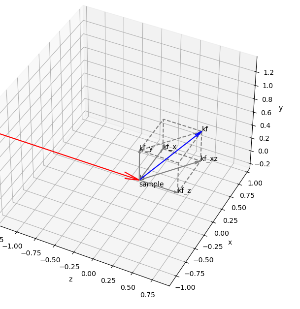
We simulate data with the calibrant LaB6
[3]:
cal = get_calibrant("LaB6")
det = Pilatus1M()
ai = AzimuthalIntegrator(detector=det, poni1=0.05, poni2=0.01, dist=0.1, wavelength=1e-10)
fake_data = cal.fake_calibration_image(ai=ai)
[4]:
jupyter.display(fake_data)
pass
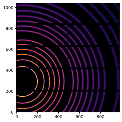
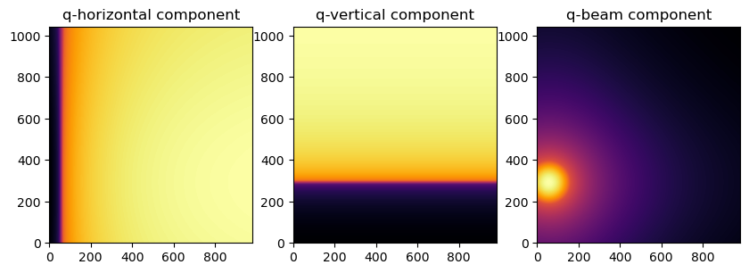
To represent the image as a function of in-plane and out-of-plane components of the q vector
[5]:
unit_qx = "qxgi_nm^-1"
unit_qy = "qygi_nm^-1"
unit_qz = "qzgi_nm^-1"
[6]:
qx = ai.array_from_unit(unit=unit_qx)
qy = ai.array_from_unit(unit=unit_qy)
qz = ai.array_from_unit(unit=unit_qz)
[7]:
fig, axes = jupyter.subplots(ncols=3, figsize=(10,5))
jupyter.display(img=qx, ax=axes[0], label="q-horizontal component")
jupyter.display(img=qy, ax=axes[1], label="q-vertical component")
jupyter.display(img=qz, ax=axes[2], label="q-beam component")
pass
[8]:
unit_qip = "qip_nm^-1"
unit_qoop = "qoop_nm^-1"
qip = ai.array_from_unit(unit=unit_qip)
qoop = ai.array_from_unit(unit=unit_qoop)
[9]:
fig, axes = jupyter.subplots(ncols=2)
jupyter.display(img=qip, ax=axes[0], label="In-plane q")
jupyter.display(img=qoop, ax=axes[1], label="Out-of-plane q")
pass
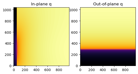
Then, GIWAXS and GISAXS patterns are represented as a function of qip and qoop
So, the horizontal component multiplied by the beam component yields the characteristic “missing wedge” of the pattern
[10]:
res2d = ai.integrate2d(fake_data, 1000,1000, unit=(unit_qip, unit_qoop), method=("no", "csr", "cython"))
jupyter.plot2d(res2d)
pass
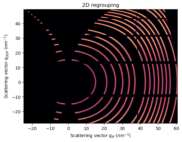
Note that is important to use a non-splitting pixel method, otherwise, the gap is filled
[11]:
res2d = ai.integrate2d(fake_data, 1000,1000, unit=(unit_qip, unit_qoop), method=("bbox", "csr", "cython"))
jupyter.plot2d(res2d)
pass
WARNING:pyFAI.geometry.core:No fast path for space: qip
WARNING:pyFAI.geometry.core:No fast path for space: qoop
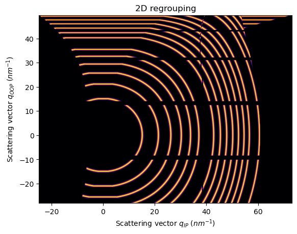
For the fiber/grazing-incidence units, pyFAI handles a special class of units called FiberUnits
FiberUnits can be retrieved with pyFAI.units.get_unit_fiber and they accept three input attributes: incident_angle, tilt_angle and sample_orientation
[12]:
unit_qip = get_unit_fiber(name="qip_nm^-1", incident_angle=0.2, tilt_angle=0.4, sample_orientation=1)
unit_qoop = get_unit_fiber(name="qoop_nm^-1", incident_angle=0.2, tilt_angle=0.4, sample_orientation=1)
ai.reset()
[13]:
res2d = ai.integrate2d(fake_data, 1000,1000, unit=(unit_qip, unit_qoop), method=("no", "csr", "cython"))
jupyter.plot2d(res2d)
pass
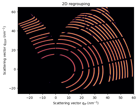
Now the patterns looks tilted due to tilt_angle and the available region in the reciprocal space has been shifted
The attribute sample_orientation takes into account the n*90 degrees difference between the fiber axis and the vertical axis of the detector
The differences are better spotted with an elongated detector
[14]:
det = RayonixLx255()
ai = AzimuthalIntegrator(detector=det, poni1=0.05, poni2=0.01, dist=0.1, wavelength=1e-10)
fake_data = cal.fake_calibration_image(ai=ai)
ai.reset()
[15]:
unit_qip.set_sample_orientation(1)
unit_qip.set_incident_angle(0.0)
unit_qip.set_tilt_angle(0.0)
unit_qoop.set_sample_orientation(1)
unit_qoop.set_incident_angle(0.0)
unit_qoop.set_tilt_angle(0.0)
ai.reset()
In this case, the incident angle goes with the short side of the detector
[16]:
res2d = ai.integrate2d(fake_data, 1000,1000, unit=(unit_qip, unit_qoop), method=("no", "csr", "cython"))
jupyter.plot2d(res2d)
pass
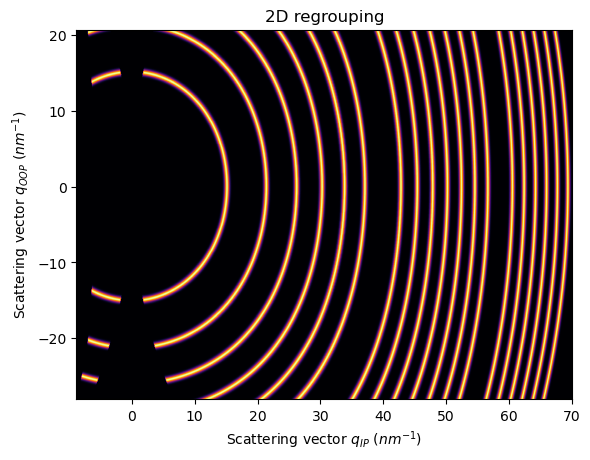
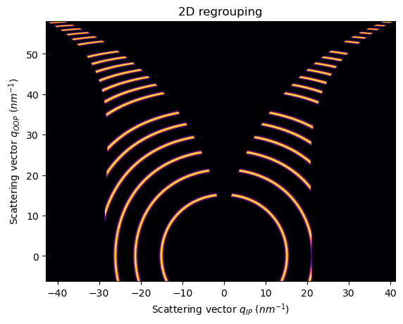
Now, if we rotate the fiber axis 90 degrees, (sample_orientation=2)
[17]:
unit_qip.set_sample_orientation(2)
unit_qoop.set_sample_orientation(2)
ai.reset()
[18]:
res2d = ai.integrate2d(fake_data, 1000,1000, unit=(unit_qip, unit_qoop), method=("no", "csr", "cython"))
jupyter.plot2d(res2d)
pass
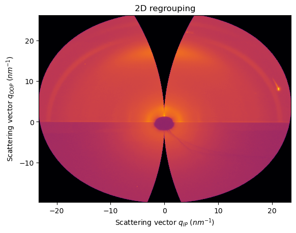
Example with real GIWAXS data
[19]:
data = fabio.open(UtilsTest.getimage("pm6.edf")).data
ai = load(UtilsTest.getimage("lab6_pm6.poni"))
We are still using sample_orientation=2
[20]:
unit_qip.sample_orientation, unit_qoop.sample_orientation
[20]:
(2, 2)
[21]:
res2d = ai.integrate2d(data, 1000,1000, unit=(unit_qip, unit_qoop), method=("no", "csr", "cython"))
jupyter.plot2d(res2d)
pass
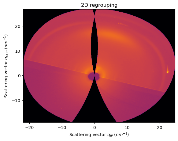
Tuning the incident and tilt angles:
[22]:
INCIDENT_ANGLE = 0.2
TILT_ANGLE = -0.3
unit_qip.set_incident_angle(INCIDENT_ANGLE)
unit_qip.set_tilt_angle(TILT_ANGLE)
unit_qoop.set_incident_angle(INCIDENT_ANGLE)
unit_qoop.set_tilt_angle(TILT_ANGLE)
ai.reset()
[23]:
res2d = ai.integrate2d(data, 1000,1000, unit=(unit_qip, unit_qoop), method=("no", "csr", "cython"))
jupyter.plot2d(res2d)
pass
Integration along a specific fiber unit
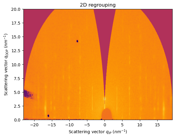
For analysis of fiber/grazing-incidence data, sometimes we need to slice the pattern along the q-oop axis, to get a set of Bragg peaks, this cannot be done using the standard cake integration
Let’s take a GIWAXS pattern collected after illuminating a crystallized semiconducting organic thin film
[24]:
data = fabio.open(UtilsTest.getimage("y6.edf")).data
ai = load(UtilsTest.getimage("LaB6_3.poni"))
INCIDENT_ANGLE = 0.0
TILT_ANGLE = 0.0
unit_qip.set_incident_angle(INCIDENT_ANGLE)
unit_qip.set_tilt_angle(TILT_ANGLE)
unit_qoop.set_incident_angle(INCIDENT_ANGLE)
unit_qoop.set_tilt_angle(TILT_ANGLE)
ai.reset()
[25]:
fig, ax = jupyter.subplots()
res2d = ai.integrate2d(data, 1000,1000, unit=(unit_qip, unit_qoop), method=("no", "csr", "cython"))
jupyter.plot2d(res2d, ax=ax)
ax.set_ylim((0,20))
pass
[26]:
cax = ax.get_children()[0]
cbar = fig.colorbar(cax)
cbar.norm.vmin = 10
cbar.norm.vmax = 1e3
ax.get_figure()
[26]:
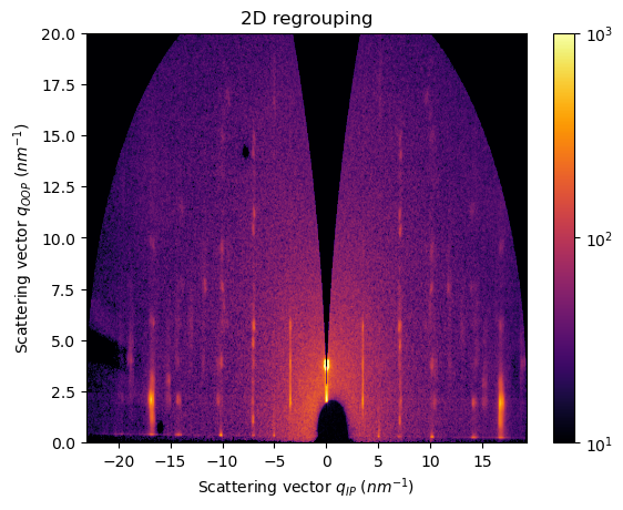
In this case, a cake integration is not accurate to capture, for example, the Bragg peaks rods at qIP=7 and 10 nm-1
Now, pyFAI allows to do this with the method pyFAI.AzimuthalIntegrator.integrate_fiber
[27]:
res_q7 = ai.integrate_fiber(data=data,
                         output_unit=unit_qoop,
                         npt_output=500,
                         output_unit_range=[0,20],
                         integrated_unit=unit_qip,
                         integrated_unit_range=[7,7.2],
                         npt_integrated=100,
                        )

res_q10 = ai.integrate_fiber(data=data,
                         output_unit=unit_qoop,
                         npt_output=500,
                         output_unit_range=[0,20],
                         integrated_unit=unit_qip,
                         integrated_unit_range=[10,10.5],
                         npt_integrated=100,
                        )
[28]:
fig, ax = jupyter.subplots()
jupyter.plot1d(res_q7, label="qIP=7", ax=ax)
jupyter.plot1d(res_q10, label="qIP=10", ax=ax)
pass
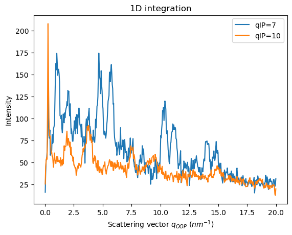
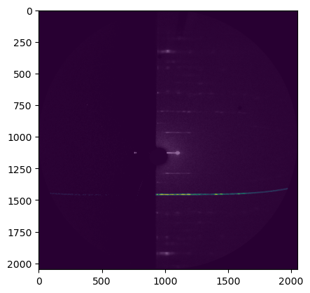
To have a clear idea of what we are integrating here, we can visualize directly the matrix
[29]:
arr_qip = ai.array_from_unit(shape=data.shape, unit=unit_qip)
arr_qoop = ai.array_from_unit(shape=data.shape, unit=unit_qoop)
arr_qip_7 = np.logical_and(arr_qip > 7.0, arr_qip < 7.2)
arr_qoop_0_20 = np.logical_and(arr_qip > 0.0, arr_qip < 20.0)
data_masked = data * arr_qip_7 * arr_qoop_0_20
[30]:
fig, ax = plt.subplots()
ax.imshow(data_masked, vmin=0, vmax=100)
ax.imshow(data, alpha=0.4, vmin=0, vmax=500, cmap="grey")
pass
[31]:
fig, ax = jupyter.subplots()
res2d = ai.integrate2d(data_masked, 1000,1000, unit=(unit_qip, unit_qoop), method=("no", "csr", "cython"))
jupyter.plot2d(res2d, ax=ax)
ax.set_ylim((0,20))
pass
[32]:
cax = ax.get_children()[0]
cbar = fig.colorbar(cax)
cbar.norm.vmin = 10
cbar.norm.vmax = 1e3
ax.get_figure()
[32]:
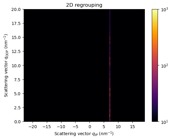
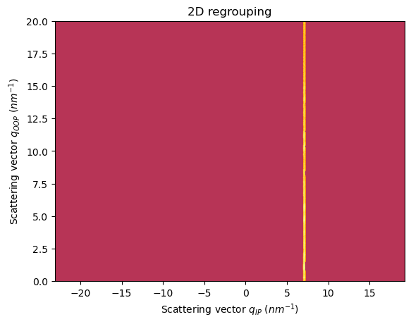
We are capturing a rectangular slice from the qip-qoop pattern, or a straight section of the Q-space in the sample frame
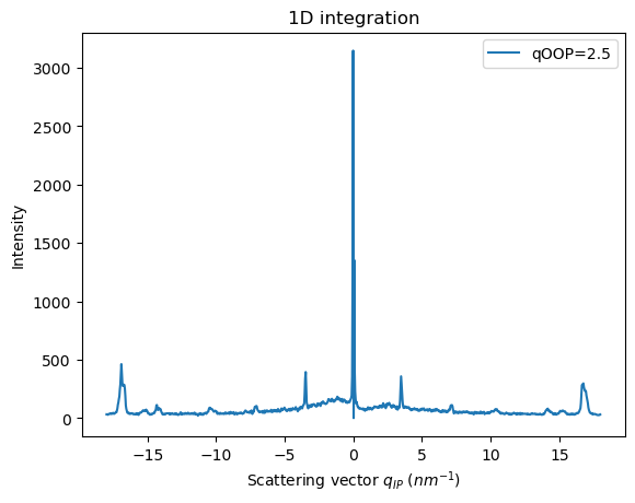
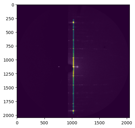
The integration is generic, we can even extract the slice along the Qoop axis
[33]:
res_q2p5 = ai.integrate_fiber(data=data,
                         output_unit=unit_qip,
                         npt_output=1000,
                         output_unit_range=[-18,18],
                         integrated_unit=unit_qoop,
                         integrated_unit_range=[2,2.5],
                         npt_integrated=100,
                        )
/home/edgar1993a/miniforge3/envs/edgar/lib/python3.11/site-packages/pyFAI/azimuthalIntegrator.py:1728: RuntimeWarning: invalid value encountered in divide
  intensity = sum_signal / sum_normalization
[34]:
fig, ax = jupyter.subplots()
jupyter.plot1d(res_q2p5, label="qOOP=2.5", ax=ax)
pass
[35]:
arr_qoop_2p5 = np.logical_and(arr_qoop > 2.0, arr_qoop < 2.5)
arr_qip_m18_18 = np.logical_and(arr_qip > -18.0, arr_qip < 18.0)
data_masked_2 = data * arr_qip_m18_18 * arr_qoop_2p5

fig, ax = plt.subplots()
ax.imshow(data_masked_2, vmin=0, vmax=100)
ax.imshow(data, alpha=0.4, vmin=0, vmax=500, cmap="grey")
pass
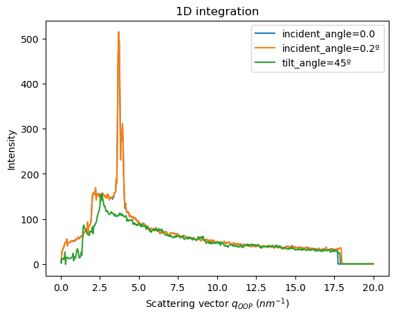
Finally, the method pyFAI.AzimuthalIntegrator.integrate_grazing_incidence allows to call the units directly with the incident_angles, tilt_angles and sample_orientation
This way, we don’t have to care about instantiating the UnitFiber and then changing the attributes
[36]:
res_1 = ai.integrate_grazing_incidence(data=data,
                                       incident_angle=0.0,
                                       tilt_angle=0.0,
                                       sample_orientation=2,
                                       output_unit="qoop_nm^-1",
                                       npt_output=500,
                                       output_unit_range=[0,20],
                                       integrated_unit="qip_nm^-1",
                                       integrated_unit_range=[-2.5,2.5],
                                       npt_integrated=100,
                                    )

res_2 = ai.integrate_grazing_incidence(data=data,
                                       incident_angle=np.deg2rad(0.2),
                                       tilt_angle=0.0,
                                       sample_orientation=2,
                                       output_unit="qoop_nm^-1",
                                       npt_output=500,
                                       output_unit_range=[0,20],
                                       integrated_unit="qip_nm^-1",
                                       integrated_unit_range=[-2.5,2.5],
                                       npt_integrated=100,
                                    )

res_3 = ai.integrate_grazing_incidence(data=data,
                                       incident_angle=np.deg2rad(0.2),
                                       tilt_angle=np.deg2rad(45),
                                       sample_orientation=2,
                                       output_unit="qoop_nm^-1",
                                       npt_output=500,
                                       output_unit_range=[0,20],
                                       integrated_unit="qip_nm^-1",
                                       integrated_unit_range=[-2.5,2.5],
                                       npt_integrated=100,
                                    )
[37]:
fig, ax = jupyter.subplots()
jupyter.plot1d(res_1, label="incident_angle=0.0", ax=ax)
jupyter.plot1d(res_2, label="incident_angle=0.2º", ax=ax)
jupyter.plot1d(res_3, label="tilt_angle=45º", ax=ax)
pass
[38]:
print(f"Total run-time: {time.perf_counter()-t0:.3f}s")
Total run-time: 37.091s
Conclusions
Now, PyFAI provides the units to represent a data array as a function of in-plane and out-of-plane components of vector q. This is a standard way of represent GIWAXS/GISAXS or fiber diffraction patterns. FiberUnits can be retrieved with a special method and the incident angle, tilt angle and sample orientation parameters can be defined and updated at the moment. Moreover, the methods integrate_fiber and integrate_grazing_incidence allow to get straight slices from the Qip-Qoop patterns.