Calibration of the pixel position for a Pilatus detector

This tutorial summarizes the work done by Frederic Sulzman during his internship at ESRF during the summer 2015 entitled “Calibration for geometric distortion in multi- modules pixel detectors”.

The overall strategy is very similar to “CCD calibration” tutorial with some specificities due to the modular nature of the detector.

0. Image preprocessing

1. Peak picking

2. Grid assignment

3. Displacement fitting

4. Reconstruction of the pixel position

5. Saving into a detector definition file

6. Validation of the geometry with a 2D integration

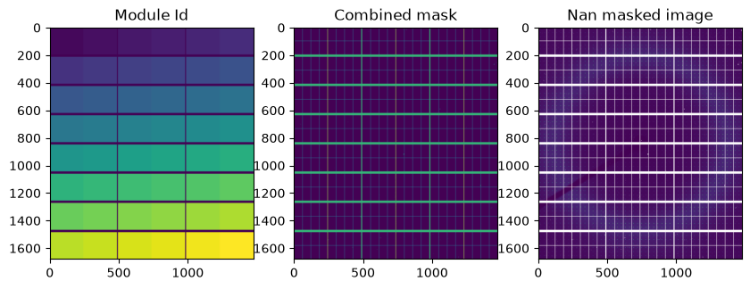
Each module being made by lithographic processes, the error within a module will be assumed to be constant. We will use the name “displacement of the module” to describe the rigid movement of the module.

This tutorial uses data from the Pilatus3 2M CdTe from the ID15 beam line of the ESRF. They provided not only the internship subject but also the couple of images used to calibrate the detector.

This detector contains 48 half-modules, each bound to a single CdTe monocrystal sensor and is designed for high energy X-ray radiation detection. Due to the construction procedure, these half-modules could show a misalignment within the detector plane. While the manufacturer (Dectris) guarantees a precision within a pixel (172µm), the misalignment of certain modules can be seen while calibrating Debye-Scherrer ring using a reference sample. So the aim of this work is to provide a detector description with a better precision than the original detector.

This work will be performed on the image of a grid available: http://www.silx.org/pub/pyFAI/detector_calibration/Pilatus2MCdTe_ID15_grid_plus_sample_0004.cbf and the scattering of ceria (CeO2) at 72.1keV available here. http://www.silx.org/pub/pyFAI/detector_calibration/Pilatus2MCdTe_ID15_CeO2_72100eV_800mm_0000.cbf

It is a good exercise to calibrate all rings of the latter image using the pyFAI-calib2 tool. A calibration close to perfection is needed to visualize the module misalignment we aim at correcting.

%matplotlib inline 
#For documentation purpose, `inline` is used to enforce the storage of the image in the notebook
#matplotlib widget
#many imports which will be used all along the notebook
import time
import pyFAI
import fabio
import numpy
from numpy.lib.stride_tricks import as_strided
from math import sin, cos, sqrt
import scipy
from scipy.ndimage import convolve, binary_dilation
from scipy.optimize import minimize
from matplotlib.pyplot import subplots
from pyFAI.ext.bilinear import Bilinear
from pyFAI.ext.watershed import InverseWatershed
from silx.resources import ExternalResources
from pyFAI.integrator.azimuthal import AzimuthalIntegrator
if scipy.__version__ >= "0.18":
    from scipy.spatial.distance  import cdist as distance_matrix
else:    
    from scipy.spatial import distance_matrix

start_time = time.perf_counter()
print("Using pyFAI verison: ", pyFAI.version)

Using pyFAI verison:  2026.9.0-dev0

# A couple of compound dtypes ...
dt = numpy.dtype([('y', numpy.float64),
                  ('x', numpy.float64),
                  ('i', numpy.int64),
                 ])
dl = numpy.dtype([('y', numpy.float64),
                  ('x', numpy.float64),
                  ('i', numpy.int64),
                  ('Y', numpy.int64),
                  ('X', numpy.int64),
                 ])

#Nota: Configure here your proxy if you are behind a firewall
#os.environ["http_proxy"] = "http://proxy.comany.com:3128"

downloader = ExternalResources("detector_calibration", "http://www.silx.org/pub/pyFAI/detector_calibration/")
ring_file = downloader.getfile("Pilatus2MCdTe_ID15_CeO2_72100eV_800mm_0000.cbf")
print(ring_file)
grid_file = downloader.getfile("Pilatus2MCdTe_ID15_grid_plus_sample_0004.cbf")
print(grid_file)

/tmp/detector_calibration_testdata_kieffer/Pilatus2MCdTe_ID15_CeO2_72100eV_800mm_0000.cbf
/tmp/detector_calibration_testdata_kieffer/Pilatus2MCdTe_ID15_grid_plus_sample_0004.cbf

rings = fabio.open(ring_file).data
img = fabio.open(grid_file).data
fig,ax = subplots(1,2, figsize=(10,5))
ax[0].imshow(img.clip(0,1000), interpolation="bilinear")
ax[0].set_title("grid")
ax[1].imshow(numpy.arcsinh(rings), interpolation="bilinear")
ax[1].set_title("rings");

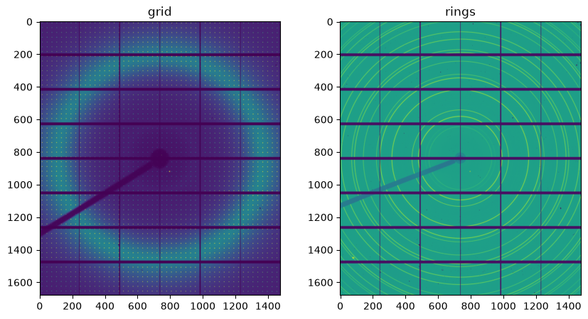
Image processing

There are 3 pre-processing steps which are needed.

1. Define for each module a unique identifier which will be used later on during the fitting procedure

2. Define the proper mask: each module is the assembly of 4x2 sub-modules and there are (3) interpolated pixels between each sub-module, such “unreliable” pixels should be masked out as well

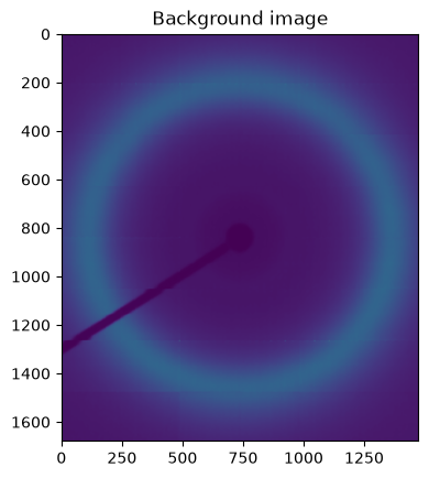
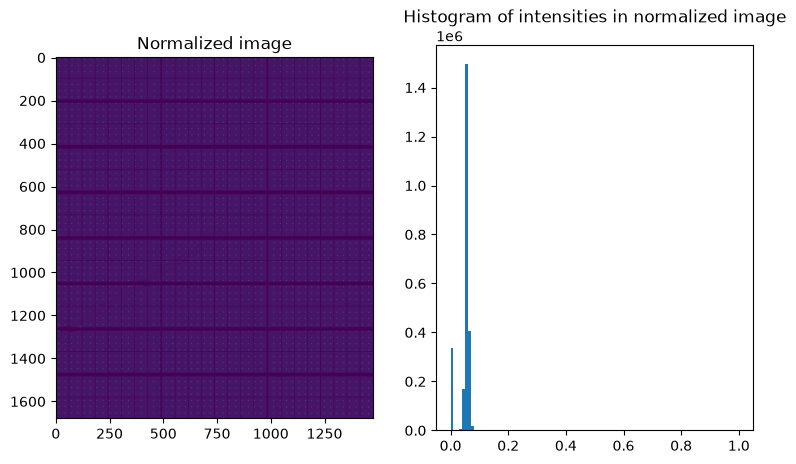
3. Correct the grid image by the smoothed image to have a constant background.

4. Convolve the raw image with a typical hole shape to allow a precise spotting of the hole center.

# This is the default detector as definied in pyFAI according to the specification provided by Dectris:
pilatus = pyFAI.detector_factory("Pilatus_2m_CdTe")
print(pilatus)

mask1 = pilatus.mask
module_size = pilatus.MODULE_SIZE
module_gap = pilatus.MODULE_GAP
submodule_size = (96,60)

Detector Pilatus CdTe 2M	 PixelSize= 172µm, 172µm	 BottomRight (3)

#1 + 2 Calculation of the module_id and the interpolated-mask:
mid = numpy.zeros(pilatus.shape, dtype=int)
mask2 = numpy.zeros(pilatus.shape, dtype=int)
idx = 1
for i in range(8):
    y_start = i*(module_gap[0] + module_size[0])
    y_stop = y_start + module_size[0]
    for j in range(3):
        x_start = j*(module_gap[1] + module_size[1])
        x_stop = x_start + module_size[1]
        mid[y_start:y_stop,x_start: x_start+module_size[1]//2] = idx
        idx+=1
        mid[y_start:y_stop,x_start+module_size[1]//2: x_stop] = idx
        idx+=1
        mask2[y_start+submodule_size[0]-1:y_start+submodule_size[0]+2,
              x_start:x_stop] = 1
        for k in range(1,8):
            mask2[y_start:y_stop,
              x_start+k*(submodule_size[1]+1)-1:x_start+k*(submodule_size[1]+1)+2] = 1

#Extra masking
mask0 = img<0
#Those pixel are miss-behaving... they are the hot pixels next to the beam-stop
mask0[915:922,793:800] = 1
mask0[817:820,747:750] = 1

fig,ax = subplots(1,3, figsize=(10,4))
ax[0].imshow(mid, interpolation="bilinear")
ax[0].set_title("Module Id")

ax[1].imshow(mask2+mask1+mask0, interpolation="bilinear")
ax[1].set_title("Combined mask")

nimg = img.astype(float)
nimg[numpy.where(mask0+mask1+mask2)] = numpy.nan


ax[2].imshow(nimg)#, interpolation="bilinear")
ax[2].set_title("Nan masked image");

# The Nan-masked image contains now only valid values (and Nan elsewhere). We will make a large median filter to 
# build up a smooth image without gaps.
#
# This function is backported from future version of numpy ... it allows to expose a winbowed view 
# to perform the nanmedian-filter

def sliding_window_view(x, shape, subok=False, readonly=True):
    """
    Creates sliding window views of the N dimensional array with the given window
    shape. Window slides across each dimension of `x` and extract subsets of `x`
    at any window position.
    Parameters
    ----------
    x : array_like
        Array to create sliding window views of.
    shape : sequence of int
        The shape of the window. Must have same length as the number of input array dimensions.
    subok : bool, optional
        If True, then sub-classes will be passed-through, otherwise the returned
        array will be forced to be a base-class array (default).
    readonly : bool, optional
        If set to True, the returned array will always be readonly view.
        Otherwise it will return writable copies(see Notes).
    Returns
    -------
    view : ndarray
        Sliding window views (or copies) of `x`. view.shape = x.shape - shape + 1
    See also
    --------
    as_strided: Create a view into the array with the given shape and strides.
    broadcast_to: broadcast an array to a given shape.
    Notes
    -----
    ``sliding_window_view`` create sliding window views of the N dimensions array
    with the given window shape and its implementation based on ``as_strided``.
    Please note that if readonly set to True, views are returned, not copies
    of array. In this case, write operations could be unpredictable, so the returned
    views are readonly. Bear in mind that returned copies (readonly=False) will
    take more memory than the original array, due to overlapping windows.
    For some cases there may be more efficient approaches to calculate transformations
    across multi-dimensional arrays, for instance `scipy.signal.fftconvolve`, where combining
    the iterating step with the calculation itself while storing partial results can result
    in significant speedups.
    Examples
    --------
    >>> i, j = np.ogrid[:3,:4]
    >>> x = 10*i + j
    >>> shape = (2,2)
    >>> np.lib.stride_tricks.sliding_window_view(x, shape)
    array([[[[ 0,  1],
             [10, 11]],
            [[ 1,  2],
             [11, 12]],
            [[ 2,  3],
             [12, 13]]],
           [[[10, 11],
             [20, 21]],
            [[11, 12],
             [21, 22]],
            [[12, 13],
             [22, 23]]]])
    """
    np = numpy
    # first convert input to array, possibly keeping subclass
    x = np.array(x, copy=False, subok=subok)

    try:
        shape = np.array(shape, dtype=np.int64)
    except Exception:
        raise TypeError('`shape` must be a sequence of integer')
    else:
        if shape.ndim > 1:
            raise ValueError('`shape` must be one-dimensional sequence of integer')
        if len(x.shape) != len(shape):
            raise ValueError("`shape` length doesn't match with input array dimensions")
        if np.any(shape <= 0):
            raise ValueError('`shape` cannot contain non-positive value')

    o = np.array(x.shape) - shape  + 1 # output shape
    if np.any(o <= 0):
        raise ValueError('window shape cannot larger than input array shape')

    if not isinstance(readonly, bool):
        raise TypeError('readonly must be a boolean')

    strides = x.strides
    view_strides = strides

    view_shape = np.concatenate((o, shape), axis=0)
    view_strides = np.concatenate((view_strides, strides), axis=0)
    view = as_strided(x, view_shape, view_strides, subok=subok, writeable=not readonly)

    if not readonly:
        return view.copy()
    else:
        return view

%%time 
#Calculate a background image using a large median filter ... takes a while
shape = (19,11)
print(nimg.shape)
padded = numpy.pad(nimg, tuple((i//2,) for i in shape), mode="edge")
print(padded.shape)
background = numpy.nanmedian(sliding_window_view(padded, shape), axis = (-2,-1))
print(background.shape)
fig,ax = subplots()
ax.imshow(background)
ax.set_title("Background image");

(1679, 1475)
(1697, 1485)
(1679, 1475)
CPU times: user 12.4 s, sys: 2.57 s, total: 15 s
Wall time: 15 s

fig,ax = subplots(1,2, figsize=(9,5))

normalized = (nimg/background)

low = numpy.nanmin(normalized)
high = numpy.nanmax(normalized)
print(low, high)
normalized[numpy.isnan(normalized)] = 0
normalized /= high

ax[0].imshow(normalized)
ax[0].set_title("Normalized image")

ax[1].hist(normalized.ravel(), 100, range=(0,1))
ax[1].set_title("Histogram of intensities in normalized image");

0.0 17.728813559322035

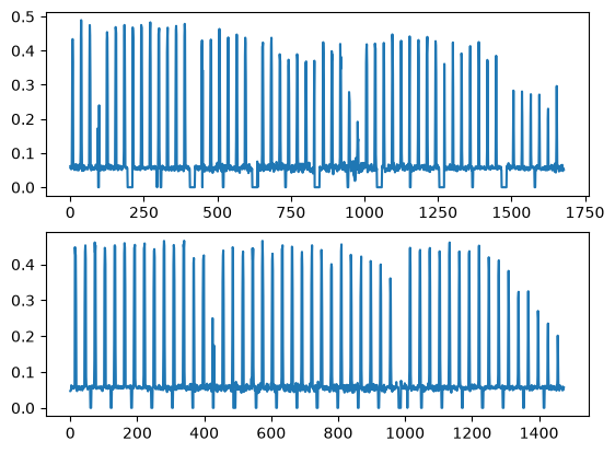
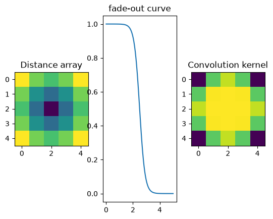
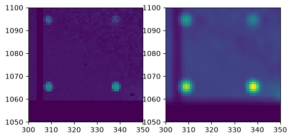
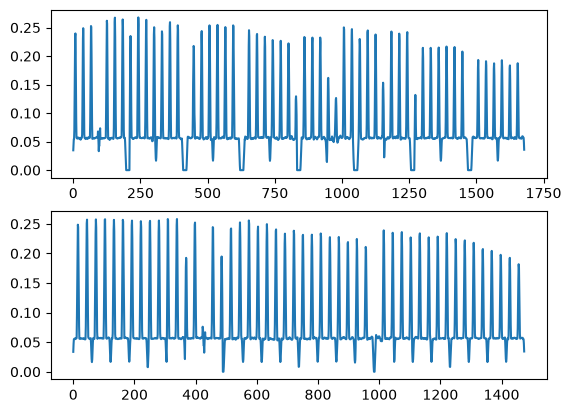
For a precise measurement of the peak position, one trick is to convolve the image with a pattern which looks like a hole of the grid.

#print the profile of the normalized image: the center is difficult to measure due to the small size of the hole.
fig,ax = subplots(2)
ax[0].plot(normalized[:,545])
ax[1].plot(normalized[536,:])
pass

#Definition of the convolution kernel
ksize = 5
y,x = numpy.ogrid[-(ksize-1)//2:ksize//2+1,-(ksize-1)//2:ksize//2+1]
d = numpy.sqrt(y*y+x*x)

#Fade out curve definition
def fadeout(x):
    return 1/(1+numpy.exp(5*(x-2.5)))

kernel = fadeout(d)
mini=kernel.sum()
print(mini)

fig,ax = subplots(1,3)
ax[0].imshow(d)
ax[0].set_title("Distance array")

ax[1].plot(numpy.linspace(0,5,100),fadeout(numpy.linspace(0,5,100)))
ax[1].set_title("fade-out curve")

ax[2].imshow(kernel)
ax[2].set_title("Convolution kernel")
pass

19.63857792789662

my_smooth = convolve(normalized, kernel, mode="constant", cval=0)/mini
print(my_smooth.shape)
fig,ax = subplots(1,2)
ax[0].imshow(normalized.clip(0,1))
ax[0].set_ylim(1050,1100)
ax[0].set_xlim(300,350)
ax[1].imshow(my_smooth.clip(0,1))
ax[1].set_ylim(1050,1100)
ax[1].set_xlim(300,350)
numpy.where(my_smooth == my_smooth.max())

(1679, 1475)

(array([1065]), array([338]))

#mask out all pixels too close to any masked position

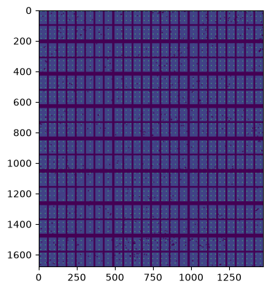
all_masks = numpy.logical_or(numpy.logical_or(mask0,mask1),mask2)
print(all_masks.sum())
big_mask = binary_dilation(all_masks, iterations=ksize//2+1+1)
print(big_mask.sum())
smooth2 = my_smooth.copy()
smooth2[big_mask] = 0
fig,ax = subplots()
ax.imshow(smooth2)
pass

335009
782371

#Display the profile of the smoothed image: the center is easy to measure thanks to the smoothness of the signal
fig,ax = subplots(2)
ax[0].plot(my_smooth[:,545])
ax[1].plot(my_smooth[536,:])
pass

Peak picking

We use the watershed module from pyFAI to retrieve all peak positions. Those regions are sieved out respectively for:

• their size, it should be larger than the kernel itself

• the peaks too close to masked regions are removed

• the intensity of the peak

iw = InverseWatershed(my_smooth)
iw.init()
iw.merge_singleton()
all_regions = set(iw.regions.values())

regions = [i for i in all_regions if i.size>mini]

print("Number of region segmented: {}".format(len(all_regions)))
print("Number of large enough regions : {}".format(len(regions)))

Number of region segmented: 82126
Number of large enough regions : 41333

#Remove peaks on masked region
sieved_region = [i for i in regions if not big_mask[(i.index//nimg.shape[-1], i.index%nimg.shape[-1])]]
print("Number of peaks not on masked areea : {}".format(len(sieved_region)))

Number of peaks not on masked areea : 30001

# Histogram of peak height:
s = numpy.array([i.maxi for i in sieved_region])

fig, ax = subplots()
ax.hist(s, 100);

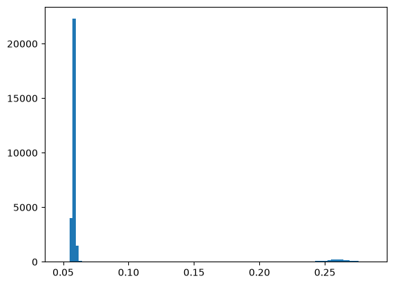
#sieve-out for peak intensity
int_mini = 0.1
peaks = [(i.index//nimg.shape[-1], i.index%nimg.shape[-1]) for i in sieved_region if (i.maxi)>int_mini]
print("Number of remaining peaks with I>{}: {}".format(int_mini, len(peaks)))

peaks_raw = numpy.array(peaks)

Number of remaining peaks with I>0.1: 2075

# Finally the peak positions are interpolated using a second order taylor expansion 
# in thevinicy of the maximum value of the signal:

#Create bilinear interpolator
bl = Bilinear(my_smooth)

#Overlay raw peak coordinate and refined peak positions

ref_peaks = [bl.local_maxi(p) for p in peaks]
fig, ax = subplots()
ax.imshow(img.clip(0,1000), interpolation="nearest")
peaks_ref = numpy.array(ref_peaks)
ax.plot(peaks_raw[:,1], peaks_raw[:, 0], ".r")
ax.plot(peaks_ref[:,1],peaks_ref[:, 0], ".b")
ax.set_title("Extracted peak position (red: raw, blue: refined)")
print("Refined peak coordinate:")
print(ref_peaks[:10])

Refined peak coordinate:
[(125.50066065788269, 662.9678415954113), (125.53483140468597, 692.4313941597939), (125.60588383674622, 721.7085201442242), (125.5032893717289, 751.2059739232063), (125.57255700230598, 780.5112820863724), (125.63533571362495, 809.9522906579077), (125.69495496153831, 839.4391780793667), (125.81450419127941, 868.7373362481594), (125.9057409465313, 898.2422359138727), (126.02405033260584, 927.544487208128)]

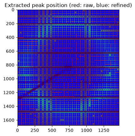
At this stage we have about 2000 peaks (with sub-pixel precision) which are visually distributed on all modules. Some modules have their peaks located along sub-module boundaries which are masked out, hence they have fewer control points for the calculation. Let’s assign each peak to a module identifier. This allows to print out the number of peaks per module:

yxi = numpy.array([i+(mid[round(i[0]),round(i[1])],) 
                   for i in ref_peaks], dtype=dt)
print("Number of keypoint per module:")
for i in range(1,mid.max()+1):
    print("Module id:",i, "cp:", (yxi[:]["i"] == i).sum())

Number of keypoint per module:
Module id: 1 cp: 48
Module id: 2 cp: 30
Module id: 3 cp: 48
Module id: 4 cp: 46
Module id: 5 cp: 42
Module id: 6 cp: 47
Module id: 7 cp: 47
Module id: 8 cp: 30
Module id: 9 cp: 48
Module id: 10 cp: 48
Module id: 11 cp: 41
Module id: 12 cp: 39
Module id: 13 cp: 48
Module id: 14 cp: 30
Module id: 15 cp: 47
Module id: 16 cp: 48
Module id: 17 cp: 42
Module id: 18 cp: 48
Module id: 19 cp: 47
Module id: 20 cp: 30
Module id: 21 cp: 48
Module id: 22 cp: 47
Module id: 23 cp: 42
Module id: 24 cp: 47
Module id: 25 cp: 48
Module id: 26 cp: 30
Module id: 27 cp: 48
Module id: 28 cp: 47
Module id: 29 cp: 41
Module id: 30 cp: 50
Module id: 31 cp: 46
Module id: 32 cp: 30
Module id: 33 cp: 48
Module id: 34 cp: 42
Module id: 35 cp: 47
Module id: 36 cp: 48
Module id: 37 cp: 48
Module id: 38 cp: 28
Module id: 39 cp: 48
Module id: 40 cp: 42
Module id: 41 cp: 44
Module id: 42 cp: 48
Module id: 43 cp: 47
Module id: 44 cp: 26
Module id: 45 cp: 46
Module id: 46 cp: 42
Module id: 47 cp: 45
Module id: 48 cp: 48

Grid assignment

The calibration is performed using a regular grid, the idea is to assign to each peak of coordinates (x,y) the integer value (X, Y) which correspond to the grid coordinate system.

The first step is to measure the grid pitch which correspond to the distance (in pixels) from one peak to the next. This is easily obtained from a pair-wise distribution function.

# pairwise distance calculation using scipy.spatial.distance_matrix

dist = distance_matrix(peaks_ref, peaks_ref)

fig, ax = subplots()
ax.hist(dist.ravel(), 100, range=(0,100))
ax.set_title("Pair-wise distribution function");

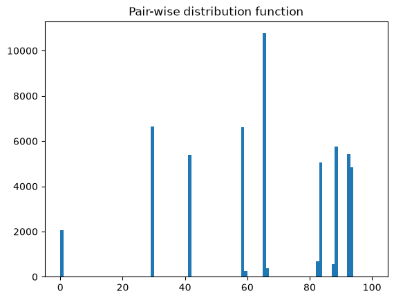
The histogram of the pair-distribution function has a first peak at 0 and the second peak between 29 and 30. Let’s start the fit with this value

Two other parameters correspond to the offset, in pixel for the grid index (X,Y) = (0,0). The easiest is to measure the smallest x and y for the first module.

#from pair-wise distribution histogram
step = 29 
#work with the first module and fit the peak positions
first = yxi[yxi[:]["i"] == 1]
y_min = first[:]["y"].min()
x_min = first[:]["x"].min()
print("offset for the first peak: ", x_min, y_min)

offset for the first peak:  16.295506536960602 7.273675739765167

The grid looks very well aligned with the axes which makes this step easier but nothing guarantees it is perfect, so the rotation of the grid has to be measured as well.

The default rotation will be zero and will be fitted later on.

Once the indexes X,Y determined for each peak, one can fit the parameter to properly align the grid with the first module. Those 4 parameters are step-size, x_min, y_min and angle

#Assign each peak to an index
indexed1 = numpy.zeros(len(first), dtype=dl)

for i,v in enumerate(first):
    Y = round((v["y"]-y_min)/step)
    X = round((v["x"]-x_min)/step)
    indexed1[i]["y"] = v["y"]
    indexed1[i]["x"] = v["x"]
    indexed1[i]["i"] = v["i"]
    indexed1[i]["Y"] = Y
    indexed1[i]["X"] = X
    print(f'peak id: {i} {v:20s} Y:{Y} (Δ={(v["y"]-Y*step-y_min)/step:.3f}) X:{X} (Δ={(v["x"]-X*step-x_min)/step:.3f})')

peak id: 0 (154.3053729236126, 16.295506536960602, 1) Y:5 (Δ=0.070) X:0 (Δ=0.000)
peak id: 1 (154.31417194008827, 45.5442131459713, 1) Y:5 (Δ=0.070) X:1 (Δ=0.009)
peak id: 2 (154.27990397810936, 75.06289485096931, 1) Y:5 (Δ=0.069) X:2 (Δ=0.026)
peak id: 3 (154.3444148004055, 104.45350721478462, 1) Y:5 (Δ=0.071) X:3 (Δ=0.040)
peak id: 4 (154.37790244817734, 133.83284245431423, 1) Y:5 (Δ=0.073) X:4 (Δ=0.053)
peak id: 5 (154.39623859524727, 163.29073610901833, 1) Y:5 (Δ=0.073) X:5 (Δ=0.069)
peak id: 6 (154.40015524625778, 192.57295206189156, 1) Y:5 (Δ=0.073) X:6 (Δ=0.079)
peak id: 7 (154.42262983322144, 222.06657180190086, 1) Y:5 (Δ=0.074) X:7 (Δ=0.096)
peak id: 8 (124.75514790415764, 16.37404641509056, 1) Y:4 (Δ=0.051) X:0 (Δ=0.003)
peak id: 9 (124.80927620828152, 45.62055751681328, 1) Y:4 (Δ=0.053) X:1 (Δ=0.011)
peak id: 10 (124.81048911809921, 75.11437203735113, 1) Y:4 (Δ=0.053) X:2 (Δ=0.028)
peak id: 11 (124.88214721530676, 104.47021272778511, 1) Y:4 (Δ=0.055) X:3 (Δ=0.041)
peak id: 12 (124.84450247883797, 133.82607851922512, 1) Y:4 (Δ=0.054) X:4 (Δ=0.053)
peak id: 13 (124.88856407254934, 163.2689579129219, 1) Y:4 (Δ=0.056) X:5 (Δ=0.068)
peak id: 14 (124.96637976542115, 192.6398860514164, 1) Y:4 (Δ=0.058) X:6 (Δ=0.081)
peak id: 15 (124.97065633907914, 222.1091116219759, 1) Y:4 (Δ=0.059) X:7 (Δ=0.097)
peak id: 16 (36.56087026000023, 16.400929421186447, 1) Y:1 (Δ=0.010) X:0 (Δ=0.004)
peak id: 17 (36.58205083012581, 45.70694240927696, 1) Y:1 (Δ=0.011) X:1 (Δ=0.014)
peak id: 18 (36.590808659791946, 75.19765095412731, 1) Y:1 (Δ=0.011) X:2 (Δ=0.031)
peak id: 19 (36.61671417951584, 104.50872442126274, 1) Y:1 (Δ=0.012) X:3 (Δ=0.042)
peak id: 20 (36.601840019226074, 133.90815691649914, 1) Y:1 (Δ=0.011) X:4 (Δ=0.056)
peak id: 21 (36.64660385251045, 163.4389183819294, 1) Y:1 (Δ=0.013) X:5 (Δ=0.074)
peak id: 22 (36.67619225382805, 192.69510865211487, 1) Y:1 (Δ=0.014) X:6 (Δ=0.083)
peak id: 23 (36.68852388858795, 222.1922933012247, 1) Y:1 (Δ=0.014) X:7 (Δ=0.100)
peak id: 24 (66.04764781147242, 16.404564529657364, 1) Y:2 (Δ=0.027) X:0 (Δ=0.004)
peak id: 25 (66.01496841665357, 45.663365960121155, 1) Y:2 (Δ=0.026) X:1 (Δ=0.013)
peak id: 26 (66.04916633665562, 75.14744073152542, 1) Y:2 (Δ=0.027) X:2 (Δ=0.029)
peak id: 27 (66.07972907274961, 104.50779458880424, 1) Y:2 (Δ=0.028) X:3 (Δ=0.042)
peak id: 28 (66.13414359092712, 133.89446383714676, 1) Y:2 (Δ=0.030) X:4 (Δ=0.055)
peak id: 29 (66.1999134272337, 163.37576597929, 1) Y:2 (Δ=0.032) X:5 (Δ=0.072)
peak id: 30 (66.15817065536976, 192.6477838754654, 1) Y:2 (Δ=0.030) X:6 (Δ=0.081)
peak id: 31 (66.13643079996109, 222.21361227333546, 1) Y:2 (Δ=0.030) X:7 (Δ=0.101)
peak id: 32 (183.53726625442505, 16.322486102581024, 1) Y:6 (Δ=0.078) X:0 (Δ=0.001)
peak id: 33 (183.58053123950958, 45.56977438926697, 1) Y:6 (Δ=0.080) X:1 (Δ=0.009)
peak id: 34 (183.6156885921955, 75.07341311872005, 1) Y:6 (Δ=0.081) X:2 (Δ=0.027)
peak id: 35 (183.62804627418518, 104.4906033873558, 1) Y:6 (Δ=0.081) X:3 (Δ=0.041)
peak id: 36 (183.68114334344864, 133.7687883079052, 1) Y:6 (Δ=0.083) X:4 (Δ=0.051)
peak id: 37 (183.68530777096748, 163.2615221142769, 1) Y:6 (Δ=0.083) X:5 (Δ=0.068)
peak id: 38 (183.67203029990196, 192.56884810328484, 1) Y:6 (Δ=0.083) X:6 (Δ=0.078)
peak id: 39 (183.75381162762642, 222.0586450919509, 1) Y:6 (Δ=0.086) X:7 (Δ=0.095)
peak id: 40 (7.309020787477493, 16.40619632601738, 1) Y:0 (Δ=0.001) X:0 (Δ=0.004)
peak id: 41 (7.273675739765167, 45.716638416051865, 1) Y:0 (Δ=0.000) X:1 (Δ=0.015)
peak id: 42 (7.303307920694351, 75.23560136556625, 1) Y:0 (Δ=0.001) X:2 (Δ=0.032)
peak id: 43 (7.322351157665253, 104.55295965075493, 1) Y:0 (Δ=0.002) X:3 (Δ=0.043)
peak id: 44 (7.279936075210571, 134.01427189446986, 1) Y:0 (Δ=0.000) X:4 (Δ=0.059)
peak id: 45 (7.34955233335495, 163.4213616847992, 1) Y:0 (Δ=0.003) X:5 (Δ=0.073)
peak id: 46 (7.396047353744507, 192.7202979028225, 1) Y:0 (Δ=0.004) X:6 (Δ=0.084)
peak id: 47 (7.381651192903519, 222.2134305536747, 1) Y:0 (Δ=0.004) X:7 (Δ=0.101)

The error in positioning each of the pixels is less than 0.1 pixel which is already excellent and will allow a straightforward fit.

The cost function for the first module is calculated as the sum of distances squared in pixel space. It uses 4 parameters which are step-size, x_min, y_min and angle

#Calculate the center of every single module for rotation around this center.
centers = {i: numpy.array([[numpy.where(mid == i)[1].mean()], [numpy.where(mid == i)[0].mean()]]) for i in range(1, 49)}
for k,v in centers.items():
    print(k,v.ravel())

1 [121.  97.]
2 [364.5  97. ]
3 [615.  97.]
4 [858.5  97. ]
5 [1109.   97.]
6 [1352.5   97. ]
7 [121. 309.]
8 [364.5 309. ]
9 [615. 309.]
10 [858.5 309. ]
11 [1109.  309.]
12 [1352.5  309. ]
13 [121. 521.]
14 [364.5 521. ]
15 [615. 521.]
16 [858.5 521. ]
17 [1109.  521.]
18 [1352.5  521. ]
19 [121. 733.]
20 [364.5 733. ]
21 [615. 733.]
22 [858.5 733. ]
23 [1109.  733.]
24 [1352.5  733. ]
25 [121. 945.]
26 [364.5 945. ]
27 [615. 945.]
28 [858.5 945. ]
29 [1109.  945.]
30 [1352.5  945. ]
31 [ 121. 1157.]
32 [ 364.5 1157. ]
33 [ 615. 1157.]
34 [ 858.5 1157. ]
35 [1109. 1157.]
36 [1352.5 1157. ]
37 [ 121. 1369.]
38 [ 364.5 1369. ]
39 [ 615. 1369.]
40 [ 858.5 1369. ]
41 [1109. 1369.]
42 [1352.5 1369. ]
43 [ 121. 1581.]
44 [ 364.5 1581. ]
45 [ 615. 1581.]
46 [ 858.5 1581. ]
47 [1109. 1581.]
48 [1352.5 1581. ]

# Define a rotation of a module around the center of the module ...

def rotate(angle, xy, module):
    "Perform the rotation of the xy points around the center of the given module"
    rot = [[cos(angle),-sin(angle)],
           [sin(angle), cos(angle)]]
    center = centers[module]
    return numpy.dot(rot, xy - center) + center

guess1 = [step, y_min, x_min, 0]

def cost1(param):
    """contains: step, y_min, x_min, angle for the first module
    returns the sum of distance squared in pixel space
    """
    step = param[0]
    y_min = param[1]
    x_min = param[2]
    angle = param[3]
    XY = numpy.vstack((indexed1["X"], indexed1["Y"]))
#     rot = [[cos(angle),-sin(angle)],
#            [sin(angle), cos(angle)]]
    xy_min = [[x_min], [y_min]]
    xy_guess = rotate(angle, step * XY + xy_min, module=1)
    delta = xy_guess - numpy.vstack((indexed1["x"], indexed1["y"]))
    return (delta*delta).sum()

print("Before optimization", guess1, "cost=", cost1(guess1))
res1 = minimize(cost1, guess1, method = "slsqp")
print(res1)
print("After optimization", res1.x, "cost=", cost1(res1.x))
print("Average displacement (pixels): ",sqrt(cost1(res1.x)/len(indexed1)))

Before optimization [29, np.float64(7.273675739765167), np.float64(16.295506536960602), 0] cost= 242.09569122473354
     message: Optimization terminated successfully
     success: True
      status: 0
         fun: 0.2728131809838241
           x: [ 2.940e+01  7.291e+00  1.631e+01  8.044e-04]
         nit: 7
         jac: [-1.218e-03 -9.272e-05 -1.592e-04 -1.268e-01]
        nfev: 50
        njev: 7
 multipliers: []
After optimization [2.93987038e+01 7.29118813e+00 1.63083343e+01 8.04405267e-04] cost= 0.2728131809838241
Average displacement (pixels):  0.07538970710357616

At this step, the grid is perfectly aligned with the first module. This module is used as the reference one and all other are aligned along it, using this first fit:

#retrieve the result of the first module fit:
step, y_min, x_min, angle = res1.x
indexed = numpy.zeros(yxi.shape, dtype=dl)

# rot =  [[cos(angle),-sin(angle)],
#         [sin(angle), cos(angle)]]
# irot =  [[cos(angle), sin(angle)],
#          [-sin(angle), cos(angle)]]

print("cost1: ",cost1([step, y_min, x_min, angle]), "for:", step, y_min, x_min, angle)

xy_min = numpy.array([[x_min], [y_min]])
xy = numpy.vstack((yxi["x"], yxi["y"]))
indexed["y"] = yxi["y"]
indexed["x"] = yxi["x"]
indexed["i"] = yxi["i"]
XY_app = (rotate(-angle, xy, 1)-xy_min) / step
XY_int = numpy.round((XY_app)).astype("int")
indexed["X"] = XY_int[0]
indexed["Y"] = XY_int[1]
xy_guess = rotate(angle, step * XY_int + xy_min, 1)

thres = 1.2
delta = abs(xy_guess - xy)
print((delta>thres).sum(), "suspicious peaks:")
suspicious = indexed[numpy.where(abs(delta>thres))[1]]
print(suspicious)

cost1:  0.2728131809838241 for: 29.39870380755854 7.291188132391677 16.30833429767888 0.0008044052670077131
26 suspicious peaks:
[(1595.48940092, 807.60422462, 46, 54, 27)
 (1595.58941016, 895.8507778 , 46, 54, 30)
 (1595.66754353, 954.58181304, 46, 54, 32)
 (1448.31671178, 748.8580925 , 40, 49, 25)
 (1448.39315033, 778.35550001, 40, 49, 26)
 (1448.49579662, 807.63068146, 40, 49, 27)
 (1448.52566186, 837.09595589, 40, 49, 28)
 (1448.58636594, 866.51127535, 40, 49, 29)
 (1448.66360906, 895.88419512, 40, 49, 30)
 (1448.90662742, 954.6377984 , 40, 49, 32)
 (1300.01775392,  14.06782181, 37, 44,  0)
 (1624.64230111, 748.83425498, 46, 55, 25)
 (1624.75863996, 807.58109996, 46, 55, 27)
 (1625.04233488, 895.79196712, 46, 55, 30)
 (1625.18665445, 954.60377797, 46, 55, 32)
 (1654.16296178, 748.69836184, 46, 56, 25)
 (1654.27297005, 778.22214852, 46, 56, 26)
 (1654.36331537, 807.50675637, 46, 56, 27)
 (1654.40003076, 836.98086103, 46, 56, 28)
 (1654.4742794 , 895.67900538, 46, 56, 30)
 (1654.49973148, 954.54310378, 46, 56, 32)
 (1419.04898635, 807.72769585, 40, 48, 27)
 (1419.30363804, 866.53197187, 40, 48, 29)
 (1419.37133303, 895.98909442, 40, 48, 30)
 (1419.50415722, 954.74084362, 40, 48, 32)
 (1566.03013446, 807.69061548, 46, 53, 27)]

fig,ax = subplots()
ax.imshow(img.clip(0,1000))
ax.plot(indexed["x"], indexed["y"],".g")
ax.plot(suspicious["x"], suspicious["y"],".r")
pass

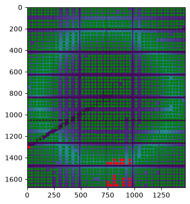
Only 6 peaks have an initial displacement of more than 1.2 pixel, all located in modules 40 and 46. The visual inspection confirms their localization is valid.

There are 48 (half-)modules which have each of them 2 translations and one rotation. In addition to the step size, this represents 145 degrees of freedom for the fit. The first module is used to align the grid, all other modules are then aligned along this grid.

def submodule_cost(param, module=1):
    """contains: step, y_min_1, x_min_1, angle_1, y_min_2, x_min_2, angle_2, ...
    returns the sum of distance squared in pixel space
    """
    
    step = param[0]
    y_min1 = param[1]
    x_min1 = param[2]
    angle1 = param[3]
    
    mask = indexed["i"] == module
    substack = indexed[mask]
    
    XY = numpy.vstack((substack["X"], substack["Y"]))
#     rot1 = [[cos(angle1), -sin(angle1)],
#             [sin(angle1), cos(angle1)]]
    xy_min1 = numpy.array([[x_min1], [y_min1]])
    xy_guess1 = rotate(angle1, step * XY + xy_min1, module=1)
    #This is guessed spot position for module #1
    if module == 1:
        "Not much to do for module 1"
        delta = xy_guess1 - numpy.vstack((substack["x"], substack["y"]))
    else:
        "perform the correction for given module"
        y_min = param[(module-1)*3+1]
        x_min = param[(module-1)*3+2]
        angle = param[(module-1)*3+3]     

#         rot = numpy.array([[cos(angle),-sin(angle)],
#                            [sin(angle), cos(angle)]])
        xy_min = numpy.array([[x_min], [y_min]])
        xy_guess = rotate(angle, xy_guess1+xy_min, module)
        delta = xy_guess - numpy.vstack((substack["x"], substack["y"]))

    return (delta*delta).sum()

guess145 = numpy.zeros(48*3+1)
guess145[:4] = res1.x
for i in range(1, 49):
    print("Cost for module #",i, submodule_cost(guess145, i))

Cost for module # 1 0.2728131809838241
Cost for module # 2 1.279477167168186
Cost for module # 3 2.043140790207666
Cost for module # 4 5.78096540171334
Cost for module # 5 1.1124684989794285
Cost for module # 6 10.230846627898266
Cost for module # 7 14.256589676943197
Cost for module # 8 4.610786323977657
Cost for module # 9 21.266725033967493
Cost for module # 10 5.617260058307791
Cost for module # 11 5.554566209658838
Cost for module # 12 9.937338353411015
Cost for module # 13 31.306238548405325
Cost for module # 14 13.207882713689239
Cost for module # 15 3.014427143099028
Cost for module # 16 6.78776245556441
Cost for module # 17 9.322752628589523
Cost for module # 18 6.458926843923407
Cost for module # 19 6.723113017277878
Cost for module # 20 5.616633921939408
Cost for module # 21 5.6308423178637925
Cost for module # 22 6.264453671812267
Cost for module # 23 1.1312733353601006
Cost for module # 24 8.454528497069598
Cost for module # 25 42.738612339600294
Cost for module # 26 22.662008754744335
Cost for module # 27 2.7919551839759924
Cost for module # 28 6.393723642568865
Cost for module # 29 14.868312741020043
Cost for module # 30 19.112748401627613
Cost for module # 31 26.89730130449964
Cost for module # 32 22.166514778164615
Cost for module # 33 17.03344033344888
Cost for module # 34 19.92677139027605
Cost for module # 35 48.468060095014515
Cost for module # 36 48.06405583860489
Cost for module # 37 73.7213097562963
Cost for module # 38 26.921069153325377
Cost for module # 39 41.4400796142651
Cost for module # 40 53.830953414309434
Cost for module # 41 21.97439738040032
Cost for module # 42 14.153821389442589
Cost for module # 43 29.021261292063446
Cost for module # 44 14.589135476796857
Cost for module # 45 51.470464222171564
Cost for module # 46 56.96490918029391
Cost for module # 47 33.79510175298672
Cost for module # 48 44.96762575356778

One retrieves that the modules 40 and 46 have large errors. Module 37 as well.

The total cost function is hence the sum of all cost functions for all modules:

def total_cost(param):
    """contains: step, y_min_1, x_min_1, angle_1, ...
    returns the sum of distance squared in pixel space
    """
    return sum(submodule_cost(param, module=i) for i in range(1,49))
total_cost(guess145)

np.float64(939.8554456072757)

%%time
print("Before optimization", guess145[:10], "cost=", total_cost(guess145))
res_all = minimize(total_cost, guess145, method = "slsqp")
print(res_all)
print("After optimization", res_all.x[:10], "cost=", total_cost(res_all.x))

Before optimization [2.93987038e+01 7.29118813e+00 1.63083343e+01 8.04405267e-04
 0.00000000e+00 0.00000000e+00 0.00000000e+00 0.00000000e+00
 0.00000000e+00 0.00000000e+00] cost= 939.8554456072757
     message: Optimization terminated successfully
     success: True
      status: 0
         fun: 13.422763294504845
           x: [ 2.941e+01  7.261e+00 ... -1.053e+00  1.837e-03]
         nit: 89
         jac: [-9.916e-01 -9.481e-03 ... -1.143e-03  3.278e-03]
        nfev: 13373
        njev: 89
 multipliers: []
After optimization [ 2.94087379e+01  7.26100614e+00  1.62732855e+01  7.54083478e-04
 -1.14589754e-01 -2.07270457e-01  2.66146289e-04  1.63761909e-01
 -2.44052715e-01  1.05284633e-03] cost= 13.422763294504845
CPU times: user 7min 56s, sys: 414 ms, total: 7min 56s
Wall time: 24.7 s

for i in range(1,49):
    print(f"Module id: {i} cost: {submodule_cost(res_all.x, i):.3f} Δx: {res_all.x[-2+i*3]:.3f}, Δy: {res_all.x[-1+i*3]:.3f} rot: {numpy.rad2deg(res_all.x[i*3]):.3f}°")

Module id: 1 cost: 0.322 Δx: 7.261, Δy: 16.273 rot: 0.043°
Module id: 2 cost: 0.196 Δx: -0.115, Δy: -0.207 rot: 0.015°
Module id: 3 cost: 0.302 Δx: 0.164, Δy: -0.244 rot: 0.060°
Module id: 4 cost: 0.261 Δx: 0.342, Δy: -0.245 rot: 0.114°
Module id: 5 cost: 0.222 Δx: 0.006, Δy: -0.473 rot: 0.029°
Module id: 6 cost: 0.295 Δx: 0.408, Δy: -0.660 rot: 0.125°
Module id: 7 cost: 0.308 Δx: -0.602, Δy: 0.060 rot: 0.088°
Module id: 8 cost: 0.153 Δx: -0.414, Δy: -0.154 rot: 0.054°
Module id: 9 cost: 0.240 Δx: -0.658, Δy: -0.432 rot: 0.059°
Module id: 10 cost: 0.267 Δx: -0.158, Δy: -0.489 rot: 0.131°
Module id: 11 cost: 0.245 Δx: 0.316, Δy: -0.286 rot: 0.031°
Module id: 12 cost: 0.255 Δx: 0.429, Δy: -0.210 rot: 0.052°
Module id: 13 cost: 0.281 Δx: -0.686, Δy: -0.604 rot: 0.068°
Module id: 14 cost: 0.145 Δx: -0.486, Δy: -0.615 rot: 0.092°
Module id: 15 cost: 0.256 Δx: -0.253, Δy: -0.375 rot: 0.062°
Module id: 16 cost: 0.208 Δx: 0.037, Δy: -0.592 rot: 0.083°
Module id: 17 cost: 0.209 Δx: -0.240, Δy: -0.807 rot: 0.038°
Module id: 18 cost: 0.390 Δx: 0.061, Δy: -0.729 rot: 0.096°
Module id: 19 cost: 0.345 Δx: -0.482, Δy: -0.278 rot: 0.053°
Module id: 20 cost: 0.176 Δx: -0.191, Δy: -0.530 rot: 0.053°
Module id: 21 cost: 0.295 Δx: -0.392, Δy: -0.465 rot: -0.016°
Module id: 22 cost: 0.276 Δx: -0.192, Δy: -0.615 rot: 0.100°
Module id: 23 cost: 0.229 Δx: -0.106, Δy: -0.358 rot: 0.078°
Module id: 24 cost: 0.551 Δx: 0.219, Δy: -0.478 rot: 0.104°
Module id: 25 cost: 0.291 Δx: -0.753, Δy: -0.851 rot: 0.059°
Module id: 26 cost: 0.157 Δx: -0.416, Δy: -0.947 rot: 0.100°
Module id: 27 cost: 0.553 Δx: -0.071, Δy: -0.297 rot: -0.028°
Module id: 28 cost: 0.279 Δx: 0.100, Δy: -0.338 rot: 0.043°
Module id: 29 cost: 0.218 Δx: -0.020, Δy: -0.929 rot: 0.037°
Module id: 30 cost: 0.609 Δx: 0.253, Δy: -0.726 rot: 0.140°
Module id: 31 cost: 0.405 Δx: -0.570, Δy: -0.777 rot: -0.035°
Module id: 32 cost: 0.410 Δx: -0.695, Δy: -0.885 rot: 0.089°
Module id: 33 cost: 0.265 Δx: -0.134, Δy: -0.777 rot: -0.022°
Module id: 34 cost: 0.191 Δx: 0.009, Δy: -0.898 rot: 0.098°
Module id: 35 cost: 0.198 Δx: -0.143, Δy: -1.390 rot: 0.048°
Module id: 36 cost: 0.382 Δx: 0.032, Δy: -1.413 rot: 0.039°
Module id: 37 cost: 0.336 Δx: -1.051, Δy: -1.137 rot: 0.002°
Module id: 38 cost: 0.129 Δx: -0.915, Δy: -0.981 rot: 0.020°
Module id: 39 cost: 0.283 Δx: -0.558, Δy: -1.148 rot: 0.014°
Module id: 40 cost: 0.228 Δx: -0.223, Δy: -1.399 rot: 0.144°
Module id: 41 cost: 0.189 Δx: -0.118, Δy: -1.051 rot: 0.024°
Module id: 42 cost: 0.289 Δx: -0.123, Δy: -0.950 rot: 0.044°
Module id: 43 cost: 0.328 Δx: -0.842, Δy: -0.772 rot: 0.058°
Module id: 44 cost: 0.132 Δx: -0.613, Δy: -0.890 rot: 0.049°
Module id: 45 cost: 0.328 Δx: -0.521, Δy: -1.298 rot: -0.009°
Module id: 46 cost: 0.316 Δx: -0.340, Δy: -1.473 rot: 0.079°
Module id: 47 cost: 0.207 Δx: -0.024, Δy: -1.149 rot: 0.074°
Module id: 48 cost: 0.276 Δx: 0.327, Δy: -1.053 rot: 0.105°

Analysis: Modules 40, 46 and 48 show large displacement but the fitting procedure allowed to reduce the residual cost to the same value as other modules.

Reconstruction of the pixel position

The pixel position can be obtained from the standard Pilatus detector. Each module is then displaced according to the fitted values, except the first one which is left where it is.

def correct(x, y, dx, dy, angle, module):
    "apply the correction dx, dy and angle to those pixels ..."
    trans = numpy.array([[dx],
                         [dy]])
    xy_guess = numpy.vstack((x.ravel(), 
                             y.ravel()))
    xy_cor = rotate(-angle, xy_guess, module) - trans
    xy_cor = xy_cor.reshape((2,)+x.shape)
    return xy_cor[0], xy_cor[1]

pixel_coord = pyFAI.detector_factory("Pilatus2MCdTe").get_pixel_corners()
pixel_coord_raw = pixel_coord.copy()
for i in range(2, 49):
    # Extract the pixel corners for one module
    module_idx = numpy.where(mid == i)
    one_module = pixel_coord_raw[module_idx]
    #retrieve the fitted values
    dy, dx, angle = res_all.x[-2+i*3:1+3*i]
    
    y = one_module[..., 1]/pilatus.pixel1
    x = one_module[..., 2]/pilatus.pixel2
    
    #apply the correction the other way around
    x_cor, y_cor = correct(x, y, dx, dy, angle, i)
    one_module[...,1] = y_cor * pilatus.pixel1 #y
    one_module[...,2] = x_cor * pilatus.pixel2 #x
    #Update the array
    pixel_coord_raw[module_idx] = one_module

Update the detector and save it in HDF5

pilatus.set_pixel_corners(pixel_coord_raw)
pilatus.mask = all_masks
pilatus.save("Pilatus_ID15_raw.h5")

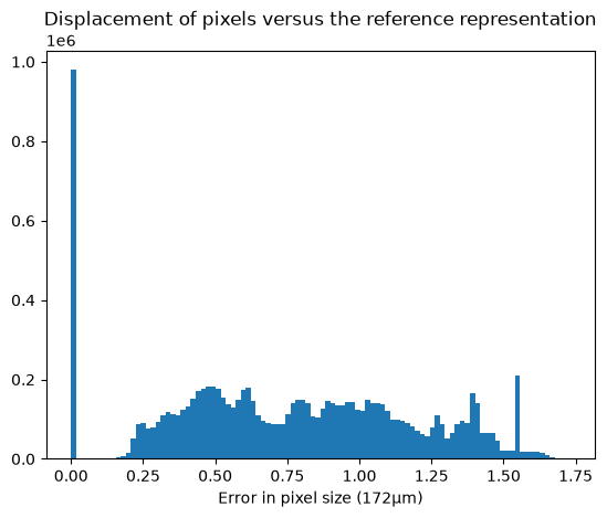
displ = numpy.sqrt(((pixel_coord - pixel_coord_raw)**2).sum(axis=-1))
displ /= pilatus.pixel1 #convert in pixel units
fig, ax = subplots()
ax.hist(displ.ravel(), 100)
ax.set_title("Displacement of pixels versus the reference representation")
ax.set_xlabel("Error in pixel size (172µm)")
pass

misaligned = numpy.vstack((pixel_coord_raw[..., 2].ravel(), #x
                           pixel_coord_raw[..., 1].ravel())) #y

reference = numpy.vstack((pixel_coord[..., 2].ravel(), #x
                          pixel_coord[..., 1].ravel())) #y

#Kabsch alignment of the whole detector ... 

def kabsch(P, R):
    "Align P on R"
    centroid_P = P.mean(axis=0)
    centroid_R = R.mean(axis=0)
    centered_P = P - centroid_P
    centered_R = R - centroid_R
    C = numpy.dot(centered_P.T, centered_R)
    V, S, W = numpy.linalg.svd(C)
    d = (numpy.linalg.det(V) * numpy.linalg.det(W)) < 0.0
    if d:
        S[-1] = -S[-1]
        V[:, -1] = -V[:, -1]
    # Create Rotation matrix U
    U = numpy.dot(V, W)
    P = numpy.dot(centered_P, U)
    return P + centroid_R
    
%time aligned = kabsch(misaligned.T, reference.T).T

CPU times: user 6.2 s, sys: 279 ms, total: 6.48 s
Wall time: 405 ms

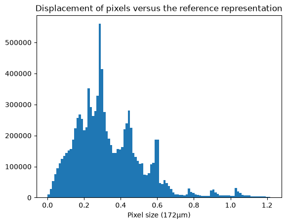
displ = numpy.sqrt(((aligned-reference)**2).sum(axis=0))
displ /= pilatus.pixel1 #convert in pixel units
fig, ax = subplots()
ax.hist(displ.ravel(), 100)
ax.set_title("Displacement of pixels versus the reference representation")
ax.set_xlabel("Pixel size (172µm)")
pass

pixel_coord_aligned = pixel_coord.copy()
pixel_coord_aligned[...,1] = aligned[1,:].reshape(pixel_coord.shape[:-1])
pixel_coord_aligned[...,2] = aligned[0,:].reshape(pixel_coord.shape[:-1])

pilatus.set_pixel_corners(pixel_coord_aligned)
pilatus.mask = all_masks
pilatus.save("Pilatus_ID15_Kabsch.h5")

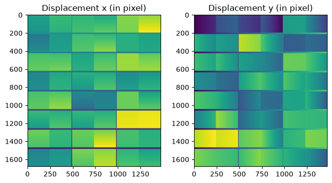
fig, ax = subplots(1, 2, figsize=(8, 4))
ax[0].imshow((pixel_coord_aligned[...,2].mean(axis=-1) - pixel_coord[...,2].mean(axis=-1))/pilatus.pixel2)
ax[0].set_title("Displacement x (in pixel)")
ax[1].imshow((pixel_coord_aligned[...,1].mean(axis=-1) - pixel_coord[...,1].mean(axis=-1))/pilatus.pixel1)
ax[1].set_title("Displacement y (in pixel)")
pass

Validation of the result

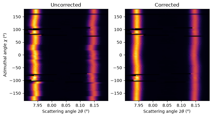
To validate the improvement obtained, one can perform the experiment calibration and the 2D integration of a reference compound, the 2D integration with either the reference from Dectris or this freshly refined detector.

# The geometry has been obtained from pyFAI
geo = { "dist":  0.8001094657585498,
        "poni1": 0.14397714477803805,
        "poni2": 0.12758748978422835,
        "rot1":  0.0011165686147339689,
        "rot2":  0.0002214091645638961,
        "rot3":  0,
        "detector": "Pilatus2MCdTe"}
ai_unc = AzimuthalIntegrator(**geo)
geo["detector"] = "Pilatus_ID15_Kabsch.h5"
ai_cor = AzimuthalIntegrator(**geo)
fig, ax = subplots(1, 2, figsize=(8,4))
method = ("pseudo", "histogram", "cython")
res_unc = ai_unc.integrate2d_ng(rings, 100, 100, radial_range=(7.9, 8.2), unit="2th_deg", method=method, mask=all_masks)
res_cor = ai_cor.integrate2d_ng(rings, 100, 100, radial_range=(7.9, 8.2), unit="2th_deg", method=method, mask=all_masks)
opts = {"origin":"lower",
        "extent": [res_unc.radial.min(), res_unc.radial.max(), -180, 180], 
        "aspect":"auto",
        "cmap":"inferno"}
ax[0].imshow(res_unc[0], **opts)
ax[1].imshow(res_cor[0], **opts)
ax[0].set_xlabel(r"Scattering angle 2$\theta$ ($^{o}$)")
ax[1].set_xlabel(r"Scattering angle 2$\theta$ ($^{o}$)")
ax[0].set_ylabel(r"Azimuthal angle $\chi$ ($^{o}$)")
ax[0].set_title("Uncorrected")
ax[1].set_title("Corrected")
pass

Conclusion

This tutorial presents the way to calibrate a module based detector using the Pilatus2M CdTe from ESRF-ID15. The HDF5 file generated is directly usable by any parts of pyFAI, the reader is invited in calibrating the rings images with the default definition and with this optimized definition and check the residual error is almost divided by a factor two.

To come back on the precision of the localization of the pixel: not all the pixels are within the specifications provided by Dectris which claims the misalignment of the modules is within one pixel.

print(f"Total execution time: {time.perf_counter()-start_time:.3f}s")

Total execution time: 54.374s