Flat-field calibration from amorphous scattering

Each pixel of an area detector has its own response: variations in sensor thickness and in charge-collection efficiency, dispersion of the read-out electronics gain and, for detectors exposed to intense beams, the progressive radiation damage of the sensor, all make the response of the detector non-uniform. The map of this response is called the flat-field, and normalizing the raw signal by it is one of the very first corrections applied to any scattering image.

Measuring a flat-field is straightforward with visible light but difficult with X-rays: it requires a uniform illumination of the whole sensor at the photon energy used for the experiment. The flood-field images provided by detector manufacturers are usually acquired at a much lower energy, where the absorption of the sensor – hence the pixel-to-pixel non-uniformity – is completely different. This is especially critical for a CdTe sensor used at high energy, and the problem gets worse with time since radiation damage keeps modifying the response of the most exposed pixels.

Weng et al. (2023) proposed an elegant way out: build the flat-field from the sample itself. The method relies on four ideas:

1. An amorphous scatterer provides a known signal. Its scattering is isotropic: it depends only on the scattering angle, not on the azimuthal angle. Once the geometrical corrections are applied (solid angle, polarization of the beam), any azimuthal variation left in the image comes from the detector.

2. The ideal image is estimated from the data themselves. A robust azimuthal average – a median rather than a mean, so that dead or damaged pixels do not bias it – provides a 1D profile I(q), which is then projected back onto the detector to produce the image an ideal detector would have recorded.

3. The ratio of the recorded and the ideal images gives the response of each pixel. This first estimate is blind wherever no data is available (beam-stop, module gaps, invalid pixels) and it is biased by anything which is not isotropic in the image: parasitic scattering, shadows, …

4. Several detector positions cure those defects. The measurement is repeated with the detector translated perpendicular to the beam: a given pixel then samples different parts of the diffraction pattern. The pixel-wise median over all positions fills the missing regions and discards the position-dependent artifacts, which appear as rings concentric to the beam-center.

The dataset used in this tutorial comes from ID31 at the ESRF: the scattering of amorphous carbon recorded at 75 keV with a Pilatus2M CdTe detector, on a grid of 9 detector positions. Each position is described by two scans: one on a silver behenate (AgBh) calibrant, used to refine the geometry, and one on the amorphous carbon, used to extract the flat-field. Compared with the original publication, where the beam was considered unpolarized, the horizontal polarization of the synchrotron beam has to be taken into account here: without this correction the signal of the amorphous scatterer is not isotropic.

Everything needed is available in pyFAI: Calibration and AbstractCalibration for the geometry, medfilt1d_ng for the median azimuthal average, calcfrom1d to project a 1D profile back onto the detector, and guess_polarization to validate the polarization factor.

Reference: J. Weng, W. Xu, K. M. Wiaderek et al., In situ X-ray area detector flat-field correction at an operating photon energy without flat illumination, J. Synchrotron Rad. (2023) 30, 546-554.

Requirements and limitations (from the original publication): the detector must have a linear response and a flat-field stable over the duration of the measurements; the scatterer must be flat (a capillary would not work, since the absorption path would depend on the azimuthal angle and not only on the scattering angle); and the beam-stop shadow must not overlap between the different detector positions.

Experimental parameters and data

The experiment was performed at 75 keV on a Pilatus2M CdTe; the calibrant is silver behenate and the beam is polarized in the horizontal plane with a factor close to 1. The 9 datasets are downloaded from silx.org and gathered in a small Position container, one per detector position.

%matplotlib inline
# Switch from widget <-> inline for documentation purposes
import copy
import time
import sys
from dataclasses import dataclass
import numpy
import h5py
from matplotlib.pyplot import subplots
import fabio
from silx.resources import ExternalResources
import pyFAI
from pyFAI.gui import jupyter
from pyFAI.gui.jupyter.calib import Calibration
from pyFAI.gui.cli_calibration import AbstractCalibration

print(f"Running pyFAI version {pyFAI.version} on python {sys.version}")
t0 = time.perf_counter()

WARNING:pyFAI.gui.matplotlib:Matplotlib already loaded with backend `inline`, setting its backend to `QtAgg` may not work!

Running pyFAI version 2026.9.0 on python 3.14.0 | packaged by conda-forge | (main, Oct 22 2025, 23:24:08) [GCC 14.3.0]

polarization = 0.999
npt = 512
energy = 75 #keV
wavelength = 1e-10*pyFAI.units.hc/energy
detector = pyFAI.detector_factory("Pilatus2M_CdTe")
calibrant = pyFAI.calibrant.CALIBRANT_FACTORY("AgBh")
calibrant.wavelength = wavelength

# Here we download the test data

downloader = ExternalResources("flatfield", "http://www.silx.org/pub/pyFAI/testimages")
all_files = downloader.getdir("flatfield_ID31.tar.bz2")
master_file = [i for i in all_files if i.endswith("calibration_0001.h5")][0]
print(master_file)

/tmp/flatfield_testdata_kieffer/flatfield_ID31.tar.bz2__content/flatfield_ID31/calibration_0001.h5

Organizing the data

All the scans are stored in a single HDF5 file following the ESRF data policy. Each detector position is described by two entries: a scan on the AgBh calibrant and a scan on the amorphous carbon. The Position dataclass below reads both images and the position of the detector stage (the cncx, cncy and cncz positioners, in millimeters), and will later hold the refined geometry, the control points and the flat-field extracted at that position.

The 9 positions are numbered from 1 to 9 and arranged on a 3x3 grid; position 5 is the central one, also available as center.

@dataclass
class Position:
    """All data related to one of the position"""    
    position: int
    calibration_idx: int
    scattering_idx: int
    coordinates: tuple=()
    calibration_data: object=None
    scattering_data: object=None
    poni: object=None
    ai: object=None
    control_points: object=None
    flatfield: object=None
    
    @classmethod
    def init(cls, h5_file, position, calibration_idx, scattering_idx, detector_name="p3", positioners=("cncx","cncy","cncz")):
        with h5py.File(h5_file) as h:
            calibration_str = f"{calibration_idx}."
            scattering_str = f"{scattering_idx}."
            keys = list(h.keys())
            ids = [i for i in keys if i.startswith(calibration_str)]
            if ids:
                entry = h[ids[0]]
                calibration_data = entry[f"measurement/{detector_name}"][0]
                coordinates = tuple(entry[f"instrument/positioners/{positioner}"][()] for positioner in positioners)
            else:
                raise IndexError(f"no such Entry {calibration_idx}")
            ids = [i for i in keys if i.startswith(scattering_str)]
            if ids:
                entry = h[ids[0]]
                scattering_data = entry[f"measurement/{detector_name}"][0]
                coordinates = tuple(entry[f"instrument/positioners/{positioner}"][()] for positioner in positioners)
            else:
                raise IndexError(f"no such Entry {calibration_idx}")
        return cls(position, calibration_idx, scattering_idx, coordinates, calibration_data, scattering_data)
            
center = Position.init(master_file, "CC", 14, 13)
center

Position(position='CC', calibration_idx=14, scattering_idx=13, coordinates=(np.float64(6489.605), np.float64(20.0), np.float64(20.0)), calibration_data=array([[2728, 2784, 2791, ..., 1582, 1636, 1544],
       [2664, 2663, 2829, ..., 1542, 1485, 1533],
       [2839, 2739, 2674, ..., 1542, 1581, 1478],
       ...,
       [3216, 2998, 3165, ..., 3048, 2992, 3125],
       [3121, 3252, 3299, ..., 3086, 3110, 2913],
       [3231, 3261, 3414, ..., 3099, 3039, 3020]],
      shape=(1679, 1475), dtype=int32), scattering_data=array([[102929, 101856, 105155, ...,  36466,  36234,  35175],
       [100320,  98901, 104158, ...,  35047,  34531,  35871],
       [102334, 101772,  98380, ...,  35634,  35428,  34703],
       ...,
       [ 96866,  94780,  96978, ...,  95870,  94463,  97045],
       [ 97101,  99105,  99604, ...,  97634,  97246,  94603],
       [100027,  99620, 102607, ...,  95336,  96377,  94539]],
      shape=(1679, 1475), dtype=int32), poni=None, ai=None, control_points=None, flatfield=None)

# This contains which scan correspond to what position and if it contains amorphous scattering or calibration data.
data =[None,
       Position.init(master_file, 1, 1, 5),
       Position.init(master_file, 2, 7, 6),
       Position.init(master_file, 3, 8, 9),
       Position.init(master_file, 4, 11, 12),
       Position.init(master_file, 5, 14, 13),
       Position.init(master_file, 6, 15, 16),
       Position.init(master_file, 7, 18, 17),
       Position.init(master_file, 8, 19, 20),
       Position.init(master_file, 9, 22, 21)]

Masking the invalid pixels

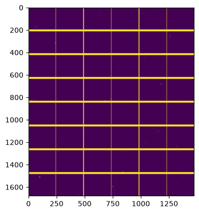
Beyond the static mask of the detector (module gaps), the pixels which are reported as negative in any of the 18 images are considered as invalid: on a Pilatus these are the dead or miscalibrated pixels flagged by the acquisition software. Taking the minimum over all images ensures that a pixel invalid in a single frame is discarded everywhere.

#calculate the mask:

mask = -detector.mask.astype(int)
for p in data[1:]:
    numpy.minimum(mask, p.scattering_data, out=mask)
    numpy.minimum(mask, p.calibration_data, out=mask)
detector.mask = (mask<0).astype(numpy.int8)
fig, ax = subplots()
ax.imshow(detector.mask)

<matplotlib.image.AxesImage at 0x7fd0844e4440>

Overview of the raw data

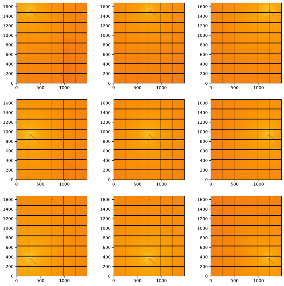
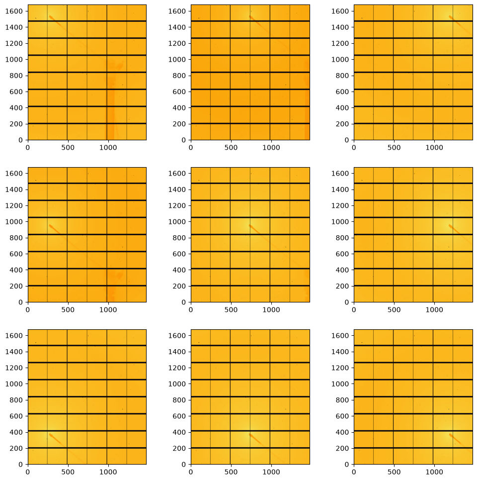
The two figures below display the 9 calibration images (AgBh rings) and the 9 amorphous carbon images. The subplots are arranged to match the actual geometry of the scan: the detector was translated perpendicular to the beam, so the diffraction pattern moves from one panel to the other. This is precisely what makes the method work – each pixel sees a different part of the pattern in each measurement.

#display calibraation scattering:
fig, ax = subplots(3,3, figsize=(12,12))
jupyter.display(data[1].calibration_data, ax=ax[0,2])
jupyter.display(data[2].calibration_data, ax=ax[0,1])
jupyter.display(data[3].calibration_data, ax=ax[0,0])
jupyter.display(data[4].calibration_data, ax=ax[1,0])
jupyter.display(data[5].calibration_data, ax=ax[1,1])
jupyter.display(data[6].calibration_data, ax=ax[1,2])
jupyter.display(data[7].calibration_data, ax=ax[2,2])
jupyter.display(data[8].calibration_data, ax=ax[2,1])
jupyter.display(data[9].calibration_data, ax=ax[2,0]);

#display amorphous scattering:
fig, ax = subplots(3,3, figsize=(12,12))
jupyter.display(data[1].scattering_data, ax=ax[0,2])
jupyter.display(data[2].scattering_data, ax=ax[0,1])
jupyter.display(data[3].scattering_data, ax=ax[0,0])
jupyter.display(data[4].scattering_data, ax=ax[1,0])
jupyter.display(data[5].scattering_data, ax=ax[1,1])
jupyter.display(data[6].scattering_data, ax=ax[1,2])
jupyter.display(data[7].scattering_data, ax=ax[2,2])
jupyter.display(data[8].scattering_data, ax=ax[2,1])
jupyter.display(data[9].scattering_data, ax=ax[2,0]);

Calibration of the central position

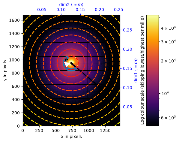
The flat-field can only be as good as the geometry used to compute it: an error on the beam-center or on the sample-detector distance would appear as a set of concentric rings in the final map.

The geometry of the central position is refined first, interactively, using the AgBh rings: switch the notebook to widget mode, then pick a few points on each ring with a right-click. Only the brightest part of the image is used here (extra_mask), since the outer rings of AgBh are too weak at 75 keV to be picked reliably.

Two peculiarities of this calibration are worth mentioning:

• the detector is known to be mounted perpendicular to the beam, so the tilt is reset to zero and rot1/rot2 are fixed during the refinement. This makes the fit much more robust when only a few rings are available;

• the mask given to the Calibration object modifies the mask of the detector itself, so the detector is deep-copied beforehand and its mask restored afterwards.

%matplotlib widget
extra_mask = center.calibration_data<5000
# switch to widget mode ... for calibration purpose. Use right click.
calib = Calibration(center.calibration_data, 
                    calibrant=calibrant, 
                    wavelength=calibrant.wavelength,
                    detector=copy.deepcopy(detector),
                    mask=extra_mask)  # Mind the mask option mangles the detector's mask ! 

input("Please perform the calibration in the previous cell before going on ... use the right-click")
%matplotlib inline
fig, ax = subplots()

#Reset the mask
calib.mask=None
calib.geoRef.detector = detector 
print(calib.geoRef)
f2d = calib.geoRef.getFit2D()
f2d["tilt"] = 0
# f2d.pop("splineFile")
print(f2d)
calib.geoRef.setFit2D(**f2d)
print(calib.geoRef)
calib.fixed += ["rot1", "rot2"]
print(calib.fixed)

Detector Pilatus CdTe 2M	 PixelSize= 172µm, 172µm	 BottomRight (3)
Wavelength= 0.165312 Å
SampleDetDist= 6.393296e+00 m	PONI= 1.533094e-01, 1.787070e-01 m	rot1=0.008172  rot2=0.001704  rot3=0.000000 rad
DirectBeamDist= 6393.519 mm	Center: x=735.220, y=954.689 pix	Tilt= 0.478° tiltPlanRotation= 168.219° λ= 0.165Å
DirectBeamDist= 6393.519 mm	Center: x=735.220, y=954.689 pix	Tilt= 0.000° tiltPlanRotation= 168.219° λ= 0.165Å
Detector Pilatus CdTe 2M	 PixelSize= 172µm, 172µm	 BottomRight (3)
Wavelength= 0.165312 Å
SampleDetDist= 6.393519e+00 m	PONI= 1.642065e-01, 1.264578e-01 m	rot1=0.000000  rot2=0.000000  rot3=0.000000 rad
DirectBeamDist= 6393.519 mm	Center: x=735.220, y=954.689 pix	Tilt= 0.000° tiltPlanRotation= 0.000° λ= 0.165Å
Fixed parameters: rot3, wavelength, rot2, rot1.

Automatic extraction of the control points

Once a first approximate geometry is known, the control points can be extracted automatically: for each expected ring, the pixels lying close to the theoretical 2θ value and brighter than the local average are used as seeds for the peak-picking. The version of extract_cpt defined below is a variant of the one shipped with pyFAI which honours the mask and limits the extraction to the max_rings first rings – only the first 4 rings of AgBh are exploitable at this energy.

logger = pyFAI.gui.cli_calibration.logger
from silx.image import marchingsquares
def extract_cpt(self, method="massif", pts_per_deg=1.0, max_rings=numpy.iinfo(int).max):
        """
        Performs an automatic keypoint extraction:
        Can be used in recalib or in calib after a first calibration has been performed.

        :param method: method for keypoint extraction
        :param pts_per_deg: number of control points per azimuthal degree (increase for better precision)
        :param max_rings: extract at most max_rings
        """
        
        logger.info("in extract_cpt with method %s", method)
        assert self.ai
        assert self.calibrant
        assert self.peakPicker
        self.peakPicker.reset()
        self.peakPicker.init(method, False)
        if self.geoRef:
            self.ai.set_config(self.geoRef.get_config())
        tth = numpy.array([i for i in self.calibrant.get_2th() if i is not None])
        tth = numpy.unique(tth)
        tth_min = numpy.zeros_like(tth)
        tth_max = numpy.zeros_like(tth)
        delta = (tth[1:] - tth[:-1]) / 4.0
        tth_max[:-1] = delta
        tth_max[-1] = delta[-1]
        tth_min[1:] = -delta
        tth_min[0] = -delta[0]
        tth_max += tth
        tth_min += tth

        shape = self.peakPicker.data.shape
        if self.geoRef:
            ttha = self.geoRef.center_array(shape, unit="2th_rad", scale=False)
            chia = self.geoRef.center_array(shape, unit="chi_rad", scale=False)
        else:
            ttha = self.ai.center_array(shape, unit="2th_rad", scale=False)
            chia = self.ai.center_array(shape, unit="chi_rad", scale=False)
        rings = 0
        self.peakPicker.sync_init()
        if self.max_rings is None:
            self.max_rings = tth.size

        ms = marchingsquares.MarchingSquaresMergeImpl(ttha, self.mask, use_minmax_cache=True)
        for i in range(tth.size):
            if rings >= min(self.max_rings, max_rings):
                break
            mask1 = numpy.logical_and(ttha >= tth_min[i], ttha < tth_max[i])
            if self.mask is not None:
                numpy.logical_and(mask1, numpy.logical_not(self.mask), out=mask1)
                
            size = mask1.sum(dtype=int)
            if (size > 0):
                rings += 1
                self.peakPicker.massif_contour(mask1)
                # if self.gui:
                #     self.peakPicker.widget.update()
                sub_data = self.peakPicker.data.ravel()[numpy.where(mask1.ravel())]
                mean = sub_data.mean(dtype=numpy.float64)
                std = sub_data.std(dtype=numpy.float64)
                upper_limit = mean + std
                mask2 = numpy.logical_and(self.peakPicker.data > upper_limit, mask1)
                size2 = mask2.sum(dtype=int)
                if size2 < 1000:
                    upper_limit = mean
                    numpy.logical_and(self.peakPicker.data > upper_limit, mask1, out=mask2)
                    size2 = mask2.sum()
                # length of the arc:
                points = ms.find_pixels(tth[i])
                seeds = {(i[0], i[1]) for i in points if mask2[i[0], i[1]]}
                # max number of points: 360 points for a full circle
                azimuthal = chia[points[:, 0].clip(0, self.peakPicker.data.shape[0]), points[:, 1].clip(0, self.peakPicker.data.shape[1])]
                nb_deg_azim = numpy.unique(numpy.rad2deg(azimuthal).round()).size
                keep = int(nb_deg_azim * pts_per_deg)
                if keep == 0:
                    continue
                dist_min = len(seeds) / 2.0 / keep
                # why 3.0, why not ?

                logger.info("Extracting datapoint for ring %s (2theta = %.2f deg); "
                            "searching for %i pts out of %i with I>%.1f, dmin=%.1f" %
                            (i, numpy.degrees(tth[i]), keep, size2, upper_limit, dist_min))
                _res = self.peakPicker.peaks_from_area(mask=mask2, Imin=upper_limit, keep=keep, method=method, ring=i, dmin=dist_min, seed=seeds)

        if self.basename:
            self.peakPicker.points.save(self.basename + ".npt")
        if self.weighted:
            self.data = self.peakPicker.points.getWeightedList(self.peakPicker.data)
        else:
            self.data = self.peakPicker.points.getList()
        if self.geoRef:
            self.geoRef.data = numpy.array(self.data, dtype=numpy.float64)
Calibration.extract_cpt = extract_cpt

calib.extract_cpt(max_rings=4)

calib.refine()

Before refinement, the geometry is:
Detector Pilatus CdTe 2M	 PixelSize= 172µm, 172µm	 BottomRight (3)
Wavelength= 0.165312 Å
SampleDetDist= 6.393519e+00 m	PONI= 1.642065e-01, 1.264578e-01 m	rot1=0.000000  rot2=0.000000  rot3=0.000000 rad
DirectBeamDist= 6393.519 mm	Center: x=735.220, y=954.689 pix	Tilt= 0.000° tiltPlanRotation= 0.000° λ= 0.165Å
Detector Pilatus CdTe 2M	 PixelSize= 172µm, 172µm	 BottomRight (3)
Wavelength= 0.165312 Å
SampleDetDist= 6.402487e+00 m	PONI= 1.642128e-01, 1.264052e-01 m	rot1=0.000000  rot2=0.000000  rot3=0.000000 rad
DirectBeamDist= 6402.487 mm	Center: x=734.914, y=954.725 pix	Tilt= 0.000° tiltPlanRotation= 0.000° λ= 0.165Å
Detector Pilatus CdTe 2M	 PixelSize= 172µm, 172µm	 BottomRight (3)
Wavelength= 0.165312 Å
SampleDetDist= 6.402487e+00 m	PONI= 1.642128e-01, 1.264052e-01 m	rot1=0.000000  rot2=0.000000  rot3=0.000000 rad
DirectBeamDist= 6402.487 mm	Center: x=734.914, y=954.725 pix	Tilt= 0.000° tiltPlanRotation= 0.000° λ= 0.165Å

From the amorphous scattering to a flat-field

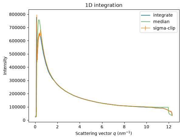
With the geometry refined, the scattering of the amorphous carbon can be azimuthally averaged. Three integration methods are compared below:

• integrate1d computes the plain mean of the pixels in each radial bin: it is sensitive to every outlier, be it a damaged pixel or a parasitic peak;

• sigma_clip iteratively removes the pixels deviating from the azimuthal average;

• medfilt1d_ng takes the median of the pixels in each bin – the most robust estimator, and the one recommended in the original publication.

All of them apply the polarization correction; guess_polarization confirms a posteriori the polarization factor by looking for the value which minimizes the azimuthal dispersion of the outer-most complete ring.

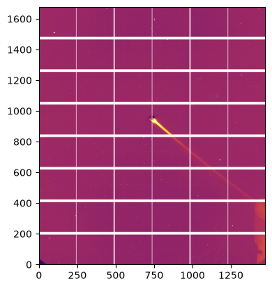
The median profile is then projected back onto the detector with calcfrom1d, which interpolates the 1D profile at the position of each pixel and re-applies the solid-angle and polarization corrections: this is the image an ideal detector would have recorded. The pixel-wise ratio between this ideal image and the measured one is the response map of the detector for this position. Masked pixels and pixels without signal are set to NaN so that they are simply ignored when the maps of the 9 positions are merged.

ai = calib.geoRef.promote("pyFAI.integrator.azimuthal.AzimuthalIntegrator")
it = ai.integrate1d(center.scattering_data, npt, polarization_factor=polarization, error_model="no", method=("no", "csr", "cython"))
sc = ai.sigma_clip(center.scattering_data, npt, polarization_factor=polarization, error_model="azimuthal", method=("no", "csr", "cython"),
                  thres=0, max_iter=3)
md = ai.medfilt1d_ng(center.scattering_data, npt, polarization_factor=polarization, method=("full", "csr", "cython"))

fig, ax = subplots()
ax = jupyter.plot1d(it, label="integrate", ax=ax)
ax.errorbar(*sc, alpha=0.7, label="sigma-clip")
ax.plot(*md, alpha=0.7, label="median")
# ax.set_yscale("log")
ax.legend();

# Approximate polarization correction needed:
print(f"Approximate polarization factor: {ai.guess_polarization(center.scattering_data, unit='q_nm^-1', target_rad=10):.4f}")

Approximate polarization factor: 0.9991

# median filter provides the smoothest curve achievable
rebuilt = ai.calcfrom1d(md.radial, 
                        md.intensity, 
                        detector.shape, 
                        dim1_unit=pyFAI.units.Q_NM, 
                        polarization_factor=polarization)
flat = rebuilt/center.scattering_data
flat[numpy.where(detector.mask)] = numpy.nan
flat[center.scattering_data<=0] = numpy.nan
jupyter.display(flat);

/tmp/ipykernel_2874142/625551917.py:7: RuntimeWarning: divide by zero encountered in divide
  flat = rebuilt/center.scattering_data

Geometry of the other positions

The map obtained above is unusable as such: it is blind under the beam-stop and in the module gaps, and it still carries the circular artifacts of anything which is not isotropic in the image. This is where the other 8 positions come into play – but each of them needs its own geometry.

Since only the detector stage was translated between the measurements, the geometry of a given position can be predicted from the central one: the displacements read from the cnc positioners (in millimeters) are simply added to poni1 and poni2 (in meters). This estimate is good enough to extract the control points automatically, and the geometry is then refined against the AgBh rings of that position – with rot1 and rot2 fixed again. The procedure is first applied step-by-step to position 1, and the refined geometry is stored, together with the geometry of the central position, in the Position containers.

dx,dy,dz = numpy.array(data[1].coordinates)-center.coordinates
ai1 = copy.copy(ai)
ai1.poni1 += dz*0.001
ai1.poni2 += dy*0.001
ai1

Detector Pilatus CdTe 2M	 PixelSize= 172µm, 172µm	 BottomRight (3)
Wavelength= 0.165312 Å
SampleDetDist= 6.402487e+00 m	PONI= 2.642128e-01, 2.051452e-01 m	rot1=0.000000  rot2=0.000000  rot3=0.000000 rad
DirectBeamDist= 6402.487 mm	Center: x=1192.705, y=1536.121 pix	Tilt= 0.000° tiltPlanRotation= 0.000° λ= 0.165Å

AbstractCalibration.extract_cpt = extract_cpt

calib1 = AbstractCalibration(data[1].calibration_data, detector.mask, detector, wavelength=wavelength, calibrant=calibrant)
calib1.preprocess()
calib1.data = []
calib1.geoRef = calib1.initgeoRef()
calib1.geoRef.set_config(ai1.get_config())

Detector Pilatus CdTe 2M	 PixelSize= 172µm, 172µm	 BottomRight (3)
Wavelength= 0.165312 Å
SampleDetDist= 6.402487e+00 m	PONI= 2.642128e-01, 2.051452e-01 m	rot1=0.000000  rot2=0.000000  rot3=0.000000 rad
DirectBeamDist= 6402.487 mm	Center: x=1192.705, y=1536.121 pix	Tilt= 0.000° tiltPlanRotation= 0.000° λ= 0.165Å

calib1.extract_cpt(max_rings=4)

ERROR:pyFAI.gui.peak_picker:No diffraction image available => not showing the contour
ERROR:pyFAI.gui.peak_picker:No diffraction image available => not showing the contour
ERROR:pyFAI.gui.peak_picker:No diffraction image available => not showing the contour
ERROR:pyFAI.gui.peak_picker:No diffraction image available => not showing the contour

calib1.fixed += ["rot1", "rot2"]
calib1.geoRef.refine3(fix=calib1.fixed)
calib1.fixed

Fixed parameters: rot3, wavelength, rot2, rot1.

calib1.geoRef

Detector Pilatus CdTe 2M	 PixelSize= 172µm, 172µm	 BottomRight (3)
Wavelength= 0.165312 Å
SampleDetDist= 6.420926e+00 m	PONI= 2.641377e-01, 2.050575e-01 m	rot1=0.000000  rot2=0.000000  rot3=0.000000 rad
DirectBeamDist= 6420.926 mm	Center: x=1192.195, y=1535.684 pix	Tilt= 0.000° tiltPlanRotation= 0.000° λ= 0.165Å

data[1].ai = pyFAI.load(calib1.geoRef)
data[1].control_points = calib1.peakPicker.points
data[5].ai = pyFAI.load(calib.geoRef)
data[5].control_points = calib.peakPicker.points

Geometry refinement for all the remaining positions

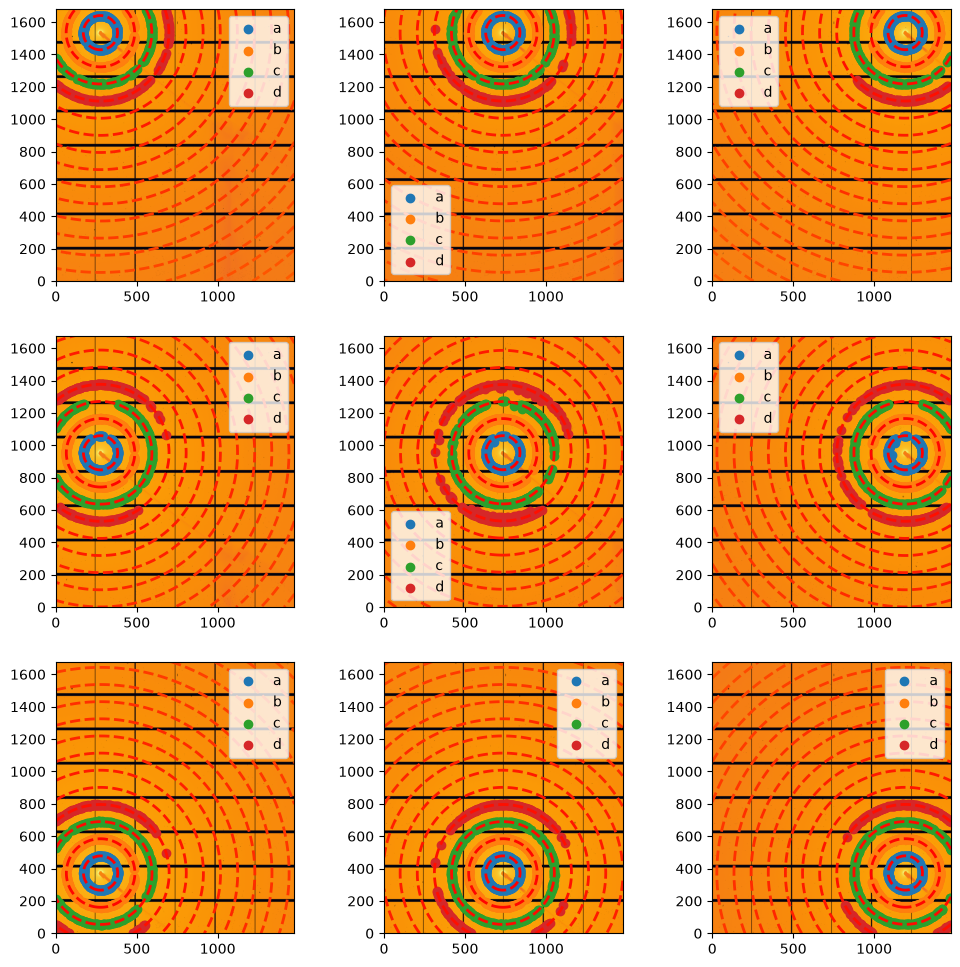
The very same recipe is now applied in a loop to the 8 remaining positions. The refined geometry and the control points used for the fit are stored in the corresponding Position object, and displayed on top of the calibration images in the figure below: the theoretical rings (in dashed lines) should overlap the measured ones over the whole detector.

for idx in [2,3,4,6,7,8,9]:
    dx,dy,dz = numpy.array(data[idx].coordinates)-center.coordinates
    ain = copy.copy(ai)
    ain.poni1 += dz*0.001
    ain.poni2 += dy*0.001
    calibn = AbstractCalibration(data[idx].calibration_data, detector.mask, detector, wavelength=wavelength, calibrant=calibrant)
    calibn.preprocess()
    calibn.data = []
    calibn.geoRef = calib1.initgeoRef()
    calibn.geoRef.set_config(ain.get_config())
    calibn.extract_cpt(max_rings=4)
    calibn.fixed += ["rot1", "rot2"]
    calibn.geoRef.refine3(fix=calibn.fixed)
    print(f"#### Position {idx} ####")
    print(calibn.geoRef)
    data[idx].ai = pyFAI.load(calibn.geoRef)
    data[idx].control_points = calibn.peakPicker.points

ERROR:pyFAI.gui.peak_picker:No diffraction image available => not showing the contour
ERROR:pyFAI.gui.peak_picker:No diffraction image available => not showing the contour
ERROR:pyFAI.gui.peak_picker:No diffraction image available => not showing the contour
ERROR:pyFAI.gui.peak_picker:No diffraction image available => not showing the contour

#### Position 2 ####
Detector Pilatus CdTe 2M	 PixelSize= 172µm, 172µm	 BottomRight (3)
Wavelength= 0.165312 Å
SampleDetDist= 6.421859e+00 m	PONI= 2.641267e-01, 1.263023e-01 m	rot1=0.000000  rot2=0.000000  rot3=0.000000 rad
DirectBeamDist= 6421.859 mm	Center: x=734.316, y=1535.620 pix	Tilt= 0.000° tiltPlanRotation= 0.000° λ= 0.165Å

ERROR:pyFAI.gui.peak_picker:No diffraction image available => not showing the contour
ERROR:pyFAI.gui.peak_picker:No diffraction image available => not showing the contour
ERROR:pyFAI.gui.peak_picker:No diffraction image available => not showing the contour
ERROR:pyFAI.gui.peak_picker:No diffraction image available => not showing the contour

#### Position 3 ####
Detector Pilatus CdTe 2M	 PixelSize= 172µm, 172µm	 BottomRight (3)
Wavelength= 0.165312 Å
SampleDetDist= 6.423568e+00 m	PONI= 2.640716e-01, 4.749240e-02 m	rot1=0.000000  rot2=0.000000  rot3=0.000000 rad
DirectBeamDist= 6423.568 mm	Center: x=276.119, y=1535.300 pix	Tilt= 0.000° tiltPlanRotation= 0.000° λ= 0.165Å

ERROR:pyFAI.gui.peak_picker:No diffraction image available => not showing the contour
ERROR:pyFAI.gui.peak_picker:No diffraction image available => not showing the contour
ERROR:pyFAI.gui.peak_picker:No diffraction image available => not showing the contour
ERROR:pyFAI.gui.peak_picker:No diffraction image available => not showing the contour

#### Position 4 ####
Detector Pilatus CdTe 2M	 PixelSize= 172µm, 172µm	 BottomRight (3)
Wavelength= 0.165312 Å
SampleDetDist= 6.424549e+00 m	PONI= 1.641524e-01, 4.763406e-02 m	rot1=0.000000  rot2=0.000000  rot3=0.000000 rad
DirectBeamDist= 6424.549 mm	Center: x=276.942, y=954.374 pix	Tilt= 0.000° tiltPlanRotation= 0.000° λ= 0.165Å

ERROR:pyFAI.gui.peak_picker:No diffraction image available => not showing the contour
ERROR:pyFAI.gui.peak_picker:No diffraction image available => not showing the contour
ERROR:pyFAI.gui.peak_picker:No diffraction image available => not showing the contour
ERROR:pyFAI.gui.peak_picker:No diffraction image available => not showing the contour

#### Position 6 ####
Detector Pilatus CdTe 2M	 PixelSize= 172µm, 172µm	 BottomRight (3)
Wavelength= 0.165312 Å
SampleDetDist= 6.424064e+00 m	PONI= 1.641631e-01, 2.051813e-01 m	rot1=0.000000  rot2=0.000000  rot3=0.000000 rad
DirectBeamDist= 6424.064 mm	Center: x=1192.915, y=954.436 pix	Tilt= 0.000° tiltPlanRotation= 0.000° λ= 0.165Å

ERROR:pyFAI.gui.peak_picker:No diffraction image available => not showing the contour
ERROR:pyFAI.gui.peak_picker:No diffraction image available => not showing the contour
ERROR:pyFAI.gui.peak_picker:No diffraction image available => not showing the contour
ERROR:pyFAI.gui.peak_picker:No diffraction image available => not showing the contour

#### Position 7 ####
Detector Pilatus CdTe 2M	 PixelSize= 172µm, 172µm	 BottomRight (3)
Wavelength= 0.165312 Å
SampleDetDist= 6.427949e+00 m	PONI= 6.421059e-02, 2.052312e-01 m	rot1=0.000000  rot2=0.000000  rot3=0.000000 rad
DirectBeamDist= 6427.949 mm	Center: x=1193.205, y=373.317 pix	Tilt= 0.000° tiltPlanRotation= 0.000° λ= 0.165Å

ERROR:pyFAI.gui.peak_picker:No diffraction image available => not showing the contour
ERROR:pyFAI.gui.peak_picker:No diffraction image available => not showing the contour
ERROR:pyFAI.gui.peak_picker:No diffraction image available => not showing the contour
ERROR:pyFAI.gui.peak_picker:No diffraction image available => not showing the contour

#### Position 8 ####
Detector Pilatus CdTe 2M	 PixelSize= 172µm, 172µm	 BottomRight (3)
Wavelength= 0.165312 Å
SampleDetDist= 6.428512e+00 m	PONI= 6.415349e-02, 1.264308e-01 m	rot1=0.000000  rot2=0.000000  rot3=0.000000 rad
DirectBeamDist= 6428.512 mm	Center: x=735.063, y=372.985 pix	Tilt= 0.000° tiltPlanRotation= 0.000° λ= 0.165Å

ERROR:pyFAI.gui.peak_picker:No diffraction image available => not showing the contour
ERROR:pyFAI.gui.peak_picker:No diffraction image available => not showing the contour
ERROR:pyFAI.gui.peak_picker:No diffraction image available => not showing the contour
ERROR:pyFAI.gui.peak_picker:No diffraction image available => not showing the contour

#### Position 9 ####
Detector Pilatus CdTe 2M	 PixelSize= 172µm, 172µm	 BottomRight (3)
Wavelength= 0.165312 Å
SampleDetDist= 6.428547e+00 m	PONI= 6.413973e-02, 4.770620e-02 m	rot1=0.000000  rot2=0.000000  rot3=0.000000 rad
DirectBeamDist= 6428.547 mm	Center: x=277.362, y=372.905 pix	Tilt= 0.000° tiltPlanRotation= 0.000° λ= 0.165Å

#display scattering:
fig, ax = subplots(3,3, figsize=(12,12))
jupyter.display(data[1].calibration_data, ai=data[1].ai, cp=data[1].control_points, ax=ax[0,2])
jupyter.display(data[2].calibration_data, ai=data[2].ai, cp=data[2].control_points, ax=ax[0,1])
jupyter.display(data[3].calibration_data, ai=data[3].ai, cp=data[3].control_points, ax=ax[0,0])
jupyter.display(data[4].calibration_data, ai=data[4].ai, cp=data[4].control_points, ax=ax[1,0])
jupyter.display(data[5].calibration_data, ai=data[5].ai, cp=data[5].control_points, ax=ax[1,1])
jupyter.display(data[6].calibration_data, ai=data[6].ai, cp=data[6].control_points, ax=ax[1,2])
jupyter.display(data[7].calibration_data, ai=data[7].ai, cp=data[7].control_points, ax=ax[2,2])
jupyter.display(data[8].calibration_data, ai=data[8].ai, cp=data[8].control_points, ax=ax[2,1])
jupyter.display(data[9].calibration_data, ai=data[9].ai, cp=data[9].control_points, ax=ax[2,0]);

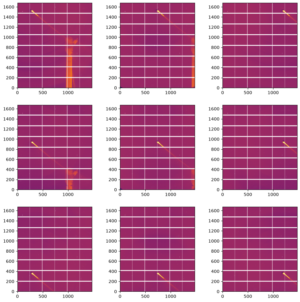
Flat-field of each individual position

Each position is now processed as the central one was: median azimuthal average of the amorphous scattering, back-projection with calcfrom1d, and pixel-wise ratio. The 9 resulting maps share the same overall structure – which is the response of the detector – but each of them has its own blind regions and its own set of concentric artifacts, centered on the beam-center of that position.

for p in data[1:]:
    md = p.ai.medfilt1d_ng(p.scattering_data, npt, polarization_factor=polarization, method=("full", "csr", "cython"))
    rebuilt = p.ai.calcfrom1d(md.radial, md.intensity, detector.shape, dim1_unit=pyFAI.units.Q_NM, polarization_factor=polarization)
    flat = rebuilt / p.scattering_data
    flat[numpy.where(detector.mask)] = numpy.nan
    flat[p.scattering_data<=0] = numpy.nan
    p.flat = flat

/tmp/ipykernel_2874142/3685900361.py:4: RuntimeWarning: divide by zero encountered in divide
  flat = rebuilt / p.scattering_data

#display flat:
fig, ax = subplots(3,3, figsize=(12,12))
jupyter.display(data[1].flat, ax=ax[0,2])
jupyter.display(data[2].flat, ax=ax[0,1])
jupyter.display(data[3].flat, ax=ax[0,0])
jupyter.display(data[4].flat, ax=ax[1,0])
jupyter.display(data[5].flat, ax=ax[1,1])
jupyter.display(data[6].flat, ax=ax[1,2])
jupyter.display(data[7].flat, ax=ax[2,2])
jupyter.display(data[8].flat, ax=ax[2,1])
jupyter.display(data[9].flat, ax=ax[2,0]);

Merging the 9 maps

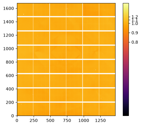
Taking the median of the 9 maps pixel-wise is what makes the artifacts disappear: the response of the detector is the same in all of them, while the artifacts are located at different places since the beam-center moved. numpy.nanmedian also takes care of the blind regions, as long as a pixel was measured at 5 positions or more.

The resulting flat-field spans roughly +/-10% around unity and clearly shows the structure of the detector modules.

flat_stack = numpy.array([p.flat for p in data[1:]])
flat = numpy.nanmedian(flat_stack, axis=0)

/tmp/ipykernel_2874142/4120576390.py:2: RuntimeWarning: All-NaN slice encountered
  flat = numpy.nanmedian(flat_stack, axis=0)

ax = jupyter.display(flat)
cb = ax.figure.colorbar(ax.images[0])
pos = numpy.linspace(0.8,1.2, 5)
ticks = [str(i) for i in pos]
cb.set_ticks(pos, labels=ticks);

Saving the result

Mind the convention: the map built above is the gain of each pixel, i.e. the ratio of the ideal signal to the measured one, as defined in the original publication where the correction is applied by multiplication. pyFAI uses the opposite convention and divides the raw signal by the flat-field: I = (raw - dark) / (flat * solidangle * polarization * absorption). This is why the reciprocal of the map is what gets saved here.

The flat-field is stored as a 32-bit float EDF image, ready to be re-used in any pyFAI processing. Keep in mind that a flat-field measured this way is only valid for the photon energy and the detector settings used here, and that it should be re-measured regularly: Weng et al. report significant changes in the response of a Pilatus2M CdTe over a couple of months. Since the whole measurement takes only a few minutes of beam time, this is affordable.

fabio.edfimage.EdfImage(data=(1/flat).astype("float32")).write("flat.edf")

print(f"Total run time: {time.perf_counter()-t0:.3f}s.")

Total run time: 274.220s.