Filtering signal in azimuthal space

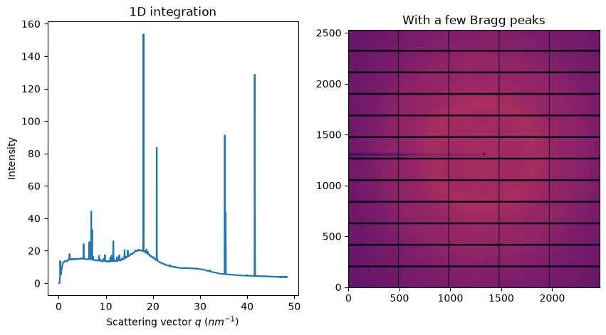
Usually, diffraction signal presents a polar symmetry, this means all pixels with the same azimuthal angle (χ) have similar intensities. The best way to exploit this is to take the mean, what is called azimuthal average. But the average is very sensitive to outliers, like gaps, missing pixels, shadows, cosmic rays or reflections coming from larger crystallites. In this tutorial we will see two alternative ways to remove those unwanted signals and focus on the majority of pixels: sigma clipping and median filtering.

import os
os.environ["PYOPENCL_COMPILER_OUTPUT"]="0"
import pyFAI
print(f"pyFAI version: {pyFAI.version}")

pyFAI version: 2026.9.0

%matplotlib inline
from matplotlib.pyplot import subplots
from pyFAI.gui import jupyter
import numpy
import fabio
from pyFAI.test.utilstest import UtilsTest
import pyFAI.benchmark

figsize = (10,5)

ai = pyFAI.load(UtilsTest.getimage("Pilatus6M.poni"))
img = fabio.open(UtilsTest.getimage("Pilatus6M.cbf")).data
fig, ax = subplots(1, 2, figsize=figsize)
jupyter.display(img, ax=ax[1])
jupyter.plot1d(ai.integrate1d(img, 1000), ax=ax[0])
ax[1].set_title("With a few Bragg peaks");

WARNING:pyFAI.gui.matplotlib:Matplotlib already loaded with backend `inline`, setting its backend to `QtAgg` may not work!

Azimuthal sigma-clipping

The idea is to discard pixels which look like outliers in the distribution of all pixels contributing to a single azimuthal bin. It requires an error model like poisson but it has been proven to be better to use the variance in the given azimuthal ring. All details are available in this publication: https://doi.org/10.1107/S1600576724011038 also available at https://doi.org/10.48550/arXiv.2411.09515

fig, ax = subplots(1, 2, figsize=figsize)
jupyter.display(img, ax=ax[1])
jupyter.plot1d(ai.sigma_clip(img, 1000, error_model="hybrid", method=("no", "csr", "cython")), ax=ax[0])
ax[1].set_title("With a few Bragg peaks")
ax[0].set_title("Sigma_clipping");

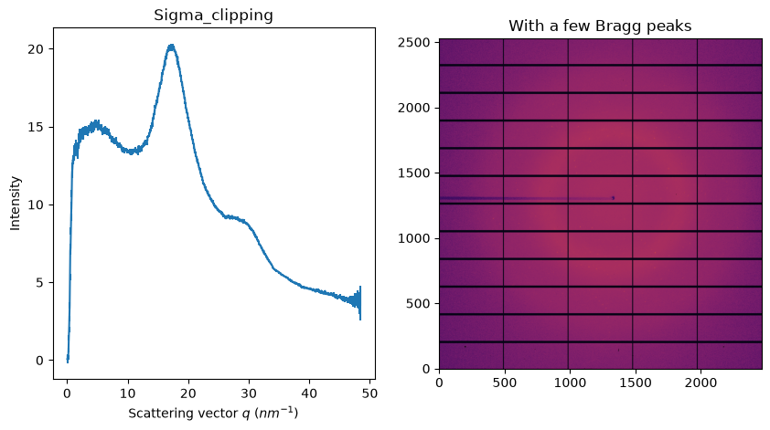
Of course, sigma-clip takes several extra parameters like the number of iterations to perform, the cut-off, the error model, … There are also a few limitations:

• The algorithm needs to be the CSR-sparse matrix multiplication: since several integrations are needed, it makes no sense to use a histogram based algorithm.

• The algorithm is available with any implementation: Python (using scipy.saprse), Cython and OpenCL, and it runs just fine on GPU.

• Sigma-clipping is incompatible with any kind of pixel splitting: With pixel splitting, a single pixel can contribute to several azimuthal bins and discarding a pixel in one ring could disable it in the neighboring ring (or not, since bins are processed in parallel).

Sigma-clipping performances:

method = ["no", "csr", "cython"]

%%time 
perfs_integrate_python = {}
perfs_integrate_cython = {}
perfs_integrate_opencl = {}
perfs_sigma_clip_python = {}
perfs_sigma_clip_cython = {}
perfs_sigma_clip_opencl = {}

for ds in pyFAI.benchmark.PONIS:
    ai = pyFAI.load(UtilsTest.getimage(ds))
    if ai.wavelength is None: ai.wavelength=1.54e-10
    img = fabio.open(UtilsTest.getimage(pyFAI.benchmark.datasets[ds])).data
    size = numpy.prod(ai.detector.shape)
    print(ds)
    print("     Cython")
    meth = tuple(method)
    nbin = max(ai.detector.shape)
    print("     * integrate ", end="")
    perfs_integrate_cython[size] = %timeit -o ai.integrate1d(img, nbin, method=meth)
    print("     * sigma-clip", end="")
    perfs_sigma_clip_cython[size] = %timeit -o ai.sigma_clip(img, nbin, method=meth, error_model="azimuthal")
    print("     Python")
    meth = tuple(method[:2]+["python"])
    print("     * integrate ", end="")
    perfs_integrate_python[size] = %timeit -o ai.integrate1d(img, nbin, method=meth)
    print("     * sigma-clip", end="")
    perfs_sigma_clip_python[size] = %timeit -o ai.sigma_clip(img, nbin, method=meth, error_model="azimuthal")

    print("     OpenCL")
    meth = tuple(method[:2]+["opencl"])
    print("     * integrate ", end="")
    perfs_integrate_opencl[size] = %timeit -o ai.integrate1d(img, nbin, method=meth)
    print("     * sigma-clip", end="")
    perfs_sigma_clip_opencl[size] = %timeit -o ai.sigma_clip(img, nbin, method=meth, error_model="azimuthal")

Pilatus1M.poni
     Cython
     * integrate 

14.5 ms ± 1.04 ms per loop (mean ± std. dev. of 7 runs, 100 loops each)
     * sigma-clip

13.4 ms ± 1.2 ms per loop (mean ± std. dev. of 7 runs, 100 loops each)
     Python
     * integrate 

10.1 ms ± 126 μs per loop (mean ± std. dev. of 7 runs, 100 loops each)
     * sigma-clip

163 ms ± 2.05 ms per loop (mean ± std. dev. of 7 runs, 10 loops each)
     OpenCL
     * integrate 

685 μs ± 1.87 μs per loop (mean ± std. dev. of 7 runs, 1,000 loops each)
     * sigma-clip

2.43 ms ± 9.09 μs per loop (mean ± std. dev. of 7 runs, 100 loops each)

Pilatus2M.poni
     Cython
     * integrate 

22.8 ms ± 2.77 ms per loop (mean ± std. dev. of 7 runs, 1 loop each)
     * sigma-clip

22.3 ms ± 2.08 ms per loop (mean ± std. dev. of 7 runs, 10 loops each)
     Python
     * integrate 

33.7 ms ± 59.1 μs per loop (mean ± std. dev. of 7 runs, 10 loops each)
     * sigma-clip

553 ms ± 1.28 ms per loop (mean ± std. dev. of 7 runs, 1 loop each)
     OpenCL
     * integrate 

1.11 ms ± 1.49 μs per loop (mean ± std. dev. of 7 runs, 1,000 loops each)
     * sigma-clip

6.06 ms ± 35.6 μs per loop (mean ± std. dev. of 7 runs, 100 loops each)
Eiger4M.poni
     Cython
     * integrate 

33.6 ms ± 2.79 ms per loop (mean ± std. dev. of 7 runs, 1 loop each)
     * sigma-clip

31.9 ms ± 872 μs per loop (mean ± std. dev. of 7 runs, 10 loops each)
     Python
     * integrate 

60.5 ms ± 199 μs per loop (mean ± std. dev. of 7 runs, 10 loops each)
     * sigma-clip

1.13 s ± 2.41 ms per loop (mean ± std. dev. of 7 runs, 1 loop each)
     OpenCL
     * integrate 

2.16 ms ± 16.8 μs per loop (mean ± std. dev. of 7 runs, 100 loops each)
     * sigma-clip

10.8 ms ± 31.6 μs per loop (mean ± std. dev. of 7 runs, 100 loops each)
Pilatus6M.poni
     Cython
     * integrate 

43 ms ± 3.01 ms per loop (mean ± std. dev. of 7 runs, 1 loop each)
     * sigma-clip

37.6 ms ± 1.9 ms per loop (mean ± std. dev. of 7 runs, 10 loops each)
     Python
     * integrate 

82.3 ms ± 541 μs per loop (mean ± std. dev. of 7 runs, 10 loops each)
     * sigma-clip

1.56 s ± 1.85 ms per loop (mean ± std. dev. of 7 runs, 1 loop each)
     OpenCL
     * integrate 

3.02 ms ± 2.87 μs per loop (mean ± std. dev. of 7 runs, 100 loops each)
     * sigma-clip

14.1 ms ± 46.3 μs per loop (mean ± std. dev. of 7 runs, 100 loops each)

Eiger9M.poni
     Cython
     * integrate 

67.5 ms ± 2.89 ms per loop (mean ± std. dev. of 7 runs, 1 loop each)
     * sigma-clip

65.6 ms ± 1.05 ms per loop (mean ± std. dev. of 7 runs, 10 loops each)
     Python
     * integrate 

150 ms ± 521 μs per loop (mean ± std. dev. of 7 runs, 10 loops each)
     * sigma-clip

3.15 s ± 4.22 ms per loop (mean ± std. dev. of 7 runs, 1 loop each)
     OpenCL
     * integrate 

4.57 ms ± 12.9 μs per loop (mean ± std. dev. of 7 runs, 100 loops each)
     * sigma-clip

25.7 ms ± 17.8 μs per loop (mean ± std. dev. of 7 runs, 10 loops each)

Mar3450.poni
     Cython
     * integrate 

66.1 ms ± 3.61 ms per loop (mean ± std. dev. of 7 runs, 1 loop each)
     * sigma-clip

69.1 ms ± 2.85 ms per loop (mean ± std. dev. of 7 runs, 10 loops each)
     Python
     * integrate 

162 ms ± 290 μs per loop (mean ± std. dev. of 7 runs, 10 loops each)
     * sigma-clip

3.51 s ± 17.2 ms per loop (mean ± std. dev. of 7 runs, 1 loop each)
     OpenCL
     * integrate 

5.24 ms ± 5.6 μs per loop (mean ± std. dev. of 7 runs, 100 loops each)
     * sigma-clip

28.9 ms ± 29.4 μs per loop (mean ± std. dev. of 7 runs, 10 loops each)

Fairchild.poni
     Cython
     * integrate 

105 ms ± 2.48 ms per loop (mean ± std. dev. of 7 runs, 1 loop each)
     * sigma-clip

122 ms ± 2.18 ms per loop (mean ± std. dev. of 7 runs, 10 loops each)
     Python
     * integrate 

378 ms ± 1.55 ms per loop (mean ± std. dev. of 7 runs, 1 loop each)
     * sigma-clip

9.63 s ± 24.8 ms per loop (mean ± std. dev. of 7 runs, 1 loop each)
     OpenCL
     * integrate 

4.91 ms ± 40 μs per loop (mean ± std. dev. of 7 runs, 1 loop each)
     * sigma-clip

33.1 ms ± 88.7 μs per loop (mean ± std. dev. of 7 runs, 10 loops each)
CPU times: user 40min 17s, sys: 39.3 s, total: 40min 56s
Wall time: 5min 42s

fig, ax = subplots()
ax.set_xlabel("Image size (Mpix)")
ax.set_ylabel("Frames per seconds")
sizes = numpy.array(list(perfs_integrate_python.keys()))/1e6
ax.plot(sizes, [1/i.best for i in perfs_integrate_python.values()], label="Integrate/Python", color='green', linestyle='dashed', marker='1')
ax.plot(sizes, [1/i.best for i in perfs_integrate_cython.values()], label="Integrate/Cython", color='orange', linestyle='dashed', marker='1')
ax.plot(sizes, [1/i.best for i in perfs_integrate_opencl.values()], label="Integrate/OpenCL", color='blue', linestyle='dashed', marker='1')
ax.plot(sizes, [1/i.best for i in perfs_sigma_clip_python.values()], label="Sigma-clip/Python", color='green', linestyle='dotted', marker='2')
ax.plot(sizes, [1/i.best for i in perfs_sigma_clip_cython.values()], label="Sigma-clip/Cython", color='orange', linestyle='dotted', marker='2')
ax.plot(sizes, [1/i.best for i in perfs_sigma_clip_opencl.values()], label="Sigma-clip/OpenCL", color='blue', linestyle='dotted', marker='2')
ax.set_yscale("log")
ax.legend()

ax.set_title("Performance of Sigma-clipping vs integrate");

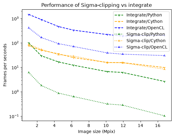
The penalty is very limited in Cython, much more in Python.

The biggest limitation of sigma-clipping is its incompatibility with pixel-splitting, a feature needed when oversampling, i.e. taking many more points than the size of the diagonal of the image. While oversampling is not recommended in the general case (due to the cross-correlation between bins it creates), it can be a necessary evil, especially when performing Rietveld refinement where 5 points per peak are needed, resolution that cannot be obtained with the pixel-size/distance couple accessible by the experimental setup.

Median filter in Azimuthal space

The idea is to sort all pixels contributing to an azimuthal bin and to average out all pixels between the lower and upper quantile. When those two thresholds are at one half, this filter provides actually the median. In order to be compatible with pixel splitting, each pixel is duplicated as many times as it contributes to different bins. After sorting fragments of pixels according to their normalization corrected signal, the cumulative sum of normalization is performed in order to determine which fragments to average out.

ai = pyFAI.load(UtilsTest.getimage("Pilatus6M.poni"))
img = fabio.open(UtilsTest.getimage("Pilatus6M.cbf")).data

method = ["full", "csr", "cython"]
percentile=(40,60)
pol=0.99

fig, ax = subplots(1, 2, figsize=figsize)
jupyter.display(img, ax=ax[1])
jupyter.plot1d(ai.medfilt1d_ng(img, 1000, method=method, percentile=percentile, polarization_factor=pol), ax=ax[0])
ax[1].set_title("With a few Bragg peaks")
ax[0].set_title("Median filtering");

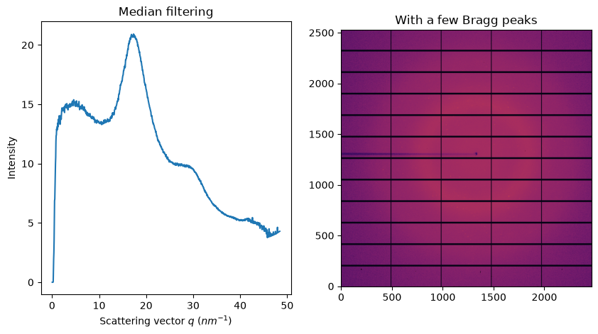
Unlike the sigma-clipping, this median filter does not require any error model; but the computational cost induced by the sort is huge. In addition, the median is very sensitive and requires a good geometry and modelisation of the polarization.

%%time 
perf2_integrate_python = {}
perf2_integrate_cython = {}
perf2_integrate_opencl = {}
perf2_medfilt_python = {}
perf2_medfilt_cython = {}
perf2_medfilt_opencl = {}

for ds in pyFAI.benchmark.PONIS:
    ai = pyFAI.load(UtilsTest.getimage(ds))
    if ai.wavelength is None: ai.wavelength=1.54e-10
    img = fabio.open(UtilsTest.getimage(pyFAI.benchmark.datasets[ds])).data
    size = numpy.prod(ai.detector.shape)
    print(ds)
    print("     Cython")
    meth = tuple(method)
    nbin = max(ai.detector.shape)
    print("     * integrate   ", end="")
    perf2_integrate_cython[size] = %timeit -o ai.integrate1d(img, nbin, method=meth)
    print("     * medianfilter", end="")
    perf2_medfilt_cython[size] = %timeit -o ai.medfilt1d_ng(img, nbin, method=meth)
    print("     Python")
    meth = tuple(method[:2]+["python"])
    print("     * integrate   ", end="")
    perf2_integrate_python[size] = %timeit -o ai.integrate1d(img, nbin, method=meth)
    print("     * medianfilter", end="")
    perf2_medfilt_python[size] = %timeit -o ai.medfilt1d_ng(img, nbin, method=meth)

    print("     OpenCL")
    meth = tuple(method[:2]+["opencl"])
    print("     * integrate   ", end="")
    perf2_integrate_opencl[size] = %timeit -o ai.integrate1d(img, nbin, method=meth)
    print("     * medianfilter", end="")
    perf2_medfilt_opencl[size] = %timeit -o ai.medfilt1d_ng(img, nbin, method=meth)

Pilatus1M.poni
     Cython
     * integrate   

19.5 ms ± 3.22 ms per loop (mean ± std. dev. of 7 runs, 1 loop each)
     * medianfilter

19.4 ms ± 2.18 ms per loop (mean ± std. dev. of 7 runs, 10 loops each)
Compiler time: 0.20 s
     Python
     * integrate   

12.8 ms ± 37.6 μs per loop (mean ± std. dev. of 7 runs, 100 loops each)
     * medianfilter

1.28 s ± 7.59 ms per loop (mean ± std. dev. of 7 runs, 1 loop each)
     OpenCL
     * integrate   

727 μs ± 1.22 μs per loop (mean ± std. dev. of 7 runs, 1,000 loops each)
     * medianfilter

9.4 ms ± 9.17 μs per loop (mean ± std. dev. of 7 runs, 100 loops each)
Pilatus2M.poni
     Cython
     * integrate   

25.7 ms ± 6.03 ms per loop (mean ± std. dev. of 7 runs, 1 loop each)
     * medianfilter

69.5 ms ± 3.47 ms per loop (mean ± std. dev. of 7 runs, 10 loops each)
     Python
     * integrate   

45.5 ms ± 248 μs per loop (mean ± std. dev. of 7 runs, 10 loops each)
     * medianfilter

4.39 s ± 49.9 ms per loop (mean ± std. dev. of 7 runs, 1 loop each)
     OpenCL
     * integrate   

1.25 ms ± 2.44 μs per loop (mean ± std. dev. of 7 runs, 1,000 loops each)
     * medianfilter

30.8 ms ± 21.7 μs per loop (mean ± std. dev. of 7 runs, 10 loops each)
Eiger4M.poni
     Cython
     * integrate   

37.1 ms ± 3.61 ms per loop (mean ± std. dev. of 7 runs, 1 loop each)
     * medianfilter

113 ms ± 633 μs per loop (mean ± std. dev. of 7 runs, 10 loops each)
     Python
     * integrate   

81.5 ms ± 88.9 μs per loop (mean ± std. dev. of 7 runs, 10 loops each)
     * medianfilter

7.41 s ± 72.5 ms per loop (mean ± std. dev. of 7 runs, 1 loop each)
     OpenCL
     * integrate   

2.34 ms ± 2.75 μs per loop (mean ± std. dev. of 7 runs, 100 loops each)
     * medianfilter

54.3 ms ± 25.8 μs per loop (mean ± std. dev. of 7 runs, 10 loops each)
Pilatus6M.poni
     Cython
     * integrate   

46.9 ms ± 3.39 ms per loop (mean ± std. dev. of 7 runs, 1 loop each)
     * medianfilter

154 ms ± 4.57 ms per loop (mean ± std. dev. of 7 runs, 10 loops each)
     Python
     * integrate   

111 ms ± 247 μs per loop (mean ± std. dev. of 7 runs, 10 loops each)
     * medianfilter

10.9 s ± 71.4 ms per loop (mean ± std. dev. of 7 runs, 1 loop each)
     OpenCL
     * integrate   

3.29 ms ± 3.13 μs per loop (mean ± std. dev. of 7 runs, 100 loops each)
     * medianfilter

78 ms ± 75.5 μs per loop (mean ± std. dev. of 7 runs, 10 loops each)

Eiger9M.poni
     Cython
     * integrate   

65.2 ms ± 2.77 ms per loop (mean ± std. dev. of 7 runs, 1 loop each)
     * medianfilter

306 ms ± 7.75 ms per loop (mean ± std. dev. of 7 runs, 1 loop each)
     Python
     * integrate   

190 ms ± 3.64 ms per loop (mean ± std. dev. of 7 runs, 1 loop each)
     * medianfilter

18.4 s ± 35.8 ms per loop (mean ± std. dev. of 7 runs, 1 loop each)
     OpenCL
     * integrate   

5.66 ms ± 1.39 ms per loop (mean ± std. dev. of 7 runs, 1 loop each)
     * medianfilter

139 ms ± 126 μs per loop (mean ± std. dev. of 7 runs, 10 loops each)

Mar3450.poni
     Cython
     * integrate   

75.4 ms ± 5.09 ms per loop (mean ± std. dev. of 7 runs, 1 loop each)
     * medianfilter

257 ms ± 2.29 ms per loop (mean ± std. dev. of 7 runs, 1 loop each)
     Python
     * integrate   

221 ms ± 849 μs per loop (mean ± std. dev. of 7 runs, 1 loop each)
     * medianfilter

21.4 s ± 183 ms per loop (mean ± std. dev. of 7 runs, 1 loop each)
     OpenCL
     * integrate   

5.94 ms ± 22.2 μs per loop (mean ± std. dev. of 7 runs, 1 loop each)
     * medianfilter

162 ms ± 191 μs per loop (mean ± std. dev. of 7 runs, 10 loops each)

Fairchild.poni
     Cython
     * integrate   

109 ms ± 3.46 ms per loop (mean ± std. dev. of 7 runs, 1 loop each)
     * medianfilter

401 ms ± 15.1 ms per loop (mean ± std. dev. of 7 runs, 1 loop each)
     Python
     * integrate   

306 ms ± 429 μs per loop (mean ± std. dev. of 7 runs, 1 loop each)
     * medianfilter

25.6 s ± 184 ms per loop (mean ± std. dev. of 7 runs, 1 loop each)
     OpenCL
     * integrate   

5.32 ms ± 34.2 μs per loop (mean ± std. dev. of 7 runs, 1 loop each)
     * medianfilter

173 ms ± 107 μs per loop (mean ± std. dev. of 7 runs, 10 loops each)
CPU times: user 25min 59s, sys: 31.9 s, total: 26min 31s
Wall time: 14min 50s

fig, ax = subplots()
ax.set_xlabel("Image size (Mpix)")
ax.set_ylabel("Frames per seconds")
sizes = numpy.array(list(perf2_integrate_python.keys()))/1e6
ax.plot(sizes, [1/i.best for i in perf2_integrate_python.values()], label="Integrate/Python", color='green', linestyle='dashed', marker='1')
ax.plot(sizes, [1/i.best for i in perf2_integrate_cython.values()], label="Integrate/Cython", color='orange', linestyle='dashed', marker='1')
ax.plot(sizes, [1/i.best for i in perf2_integrate_opencl.values()], label="Integrate/OpenCL", color='blue', linestyle='dashed', marker='1')
ax.plot(sizes, [1/i.best for i in perf2_medfilt_python.values()], label="Medfilt/Python", color='green', linestyle='dotted', marker='2')
ax.plot(sizes, [1/i.best for i in perf2_medfilt_cython.values()], label="Medfilt/Cython", color='orange', linestyle='dotted', marker='2')
ax.plot(sizes, [1/i.best for i in perf2_medfilt_opencl.values()], label="Medfilt/OpenCL", color='blue', linestyle='dotted', marker='2')
ax.set_yscale("log")
ax.legend()
ax.set_title("Performance of Median filtering vs integrate");

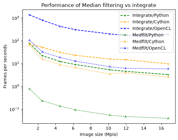
As one can see, the penalties are much larger for OpenCL and Python than for Cython.

Conclusion

Sigma-clipping and median-filtering are alternatives to azimuthal integration and offer the ability to reject outliers. They are not more difficult to use but slightly slower owing to their greater complexity.