Calibration of modular detectors using Debye-Scherrer rings#
Large pixel detectors are not monolithic: they are assembled from individual modules, each of them nearly perfect since produced by lithography, but positioned with the tolerance of a mechanical assembly. The resulting misalignments are small — a fraction of a pixel — yet they are large enough to show up as steps in the position of the powder rings at the module boundaries, and to limit the accuracy of any strain measurement performed with such a detector.
The usual way to characterize this distortion is to image a calibration object, typically a metal plate drilled with a grid of holes. This has two limitations: the machining tolerance of the object itself, and the fact that the grid only samples the distortion at its nodes, which restricts the correction to its low-frequency components.
The method demonstrated in this tutorial replaces the grid by the diffraction signal itself. Debye-Scherrer rings are continuous, they are recorded through the very same optical path as the data, and they cover the whole surface of the detector: this gives access to all spatial frequencies of the distortion. Several images are recorded with different beam-center positions, so that every module sees rings at various places, and a single least-squares fit refines simultaneously the position of every module (2 translations and 1 rotation each) and the experimental geometry of every image.
Developed initially by Jonathan P. Wright, Carlotta Giacobbe and Eleanor Lawrence Bright from ESRF-ID11 in https://doi.org/10.3390/cryst12020255, the method is applied here to the Eiger2 CdTe 4M of ID11, and its outcome is compared with the tabulated geometry of the detector and with the geometry measured from a grid of holes.
Images can be obtained from:
https://www.silx.org/pub/pyFAI/detector_calibration/Eiger2-ID11/CeO2_Spatial_distortion_apr2021.tar.bz2
In this tutorial, we start from the control-points used for calibrating the detector position for all 4
geometries, using for instance pyFAI-calib2 on each of the 4 images available in the archive.
Once the geometry optained with good confidence, return to the third tab called “Peak picking”.
Select and click “Extract all rings”.
Tune the “Number of peaks per degree” as high as the quality of your data permits, stop when out-of-ring control-point get picked.
For this tutorial, control points and PONIs needs to be saved in files with the same basename, respectively in the third and fith tab of pyFAI-calib2).
%matplotlib inline
import glob
import os
import time
from matplotlib.pyplot import subplots
from IPython.display import Markdown
import numpy
import pyFAI
from pyFAI.gui import jupyter
from pyFAI.control_points import ControlPoints
from pyFAI.goniometer import SingleGeometry
from pyFAI.detectors.multi_module import MultiModuleRefinement
from pyFAI.utils.grid import Kabsch
print(f"Using pyFAI version {pyFAI.version}")
start_time = time.perf_counter()
Using pyFAI version 2026.9.0
ponis = glob.glob("*.poni")
ponis.sort()
cpf = glob.glob("*.npt")
cpf.sort()
tabulated_detector = pyFAI.detector_factory("Eiger2_CdTe_4M")
print("Control-points files: "+ ", ".join(cpf))
print("Total number of control-points: ", sum( len(ControlPoints(c).getListRing()) for i, c in enumerate(cpf)))
Control-points files: geom_0001.npt, geom_0002.npt, geom_0003.npt, geom_0004.npt
Total number of control-points:  62136
fig, ax = subplots(2,2, figsize=(10,8))

shape = pyFAI.load(ponis[0]).detector.shape
for i, c in enumerate(cpf):
    img = numpy.zeros(tabulated_detector.shape)
    img[tabulated_detector.mask>0] = numpy.nan
    cp = ControlPoints(c)
    y, x, n = numpy.array(cp.getList()).T
    ax[i//2, i%2].imshow(img, origin="lower")
    ax[i//2, i%2].set_title(c)
    ax[i//2, i%2].scatter(x, y, 1, c=n)
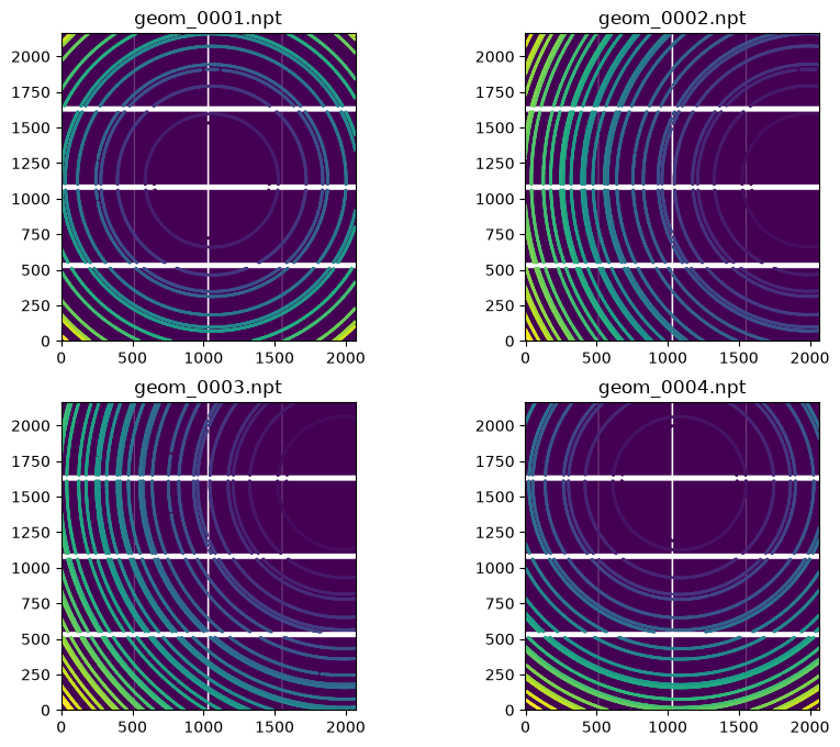
The four calibration images, with their control points colored by ring index: the beam center moves from one image to the next, so that each block of pixels sees rings at different places.
# Visualization of the need for calibration of module position
ring_idx = 0  # ring number

fig,ax = subplots()
for i, (c,p) in enumerate(zip(cpf, ponis)):
    ai = pyFAI.load(p)
    cp = pyFAI.control_points.ControlPoints(c)
    ring = numpy.array([(d[0], d[1]) for d in cp.getListRing() if d[2] == ring_idx])
    d0, d1 = ring.T
    tth = numpy.rad2deg(ai.tth(d0, d1))
    chi = numpy.rad2deg(ai.chi(d0, d1))
    ax.scatter(chi, tth, s=1)
ax.set_xlabel(r"Azimthal angle ($\chi ^o$)")
ax.set_ylabel(r"Radial angle (2$\theta ^o$)")
ax.set_title(f"Spread of radial angle for ring #{ring_idx}");
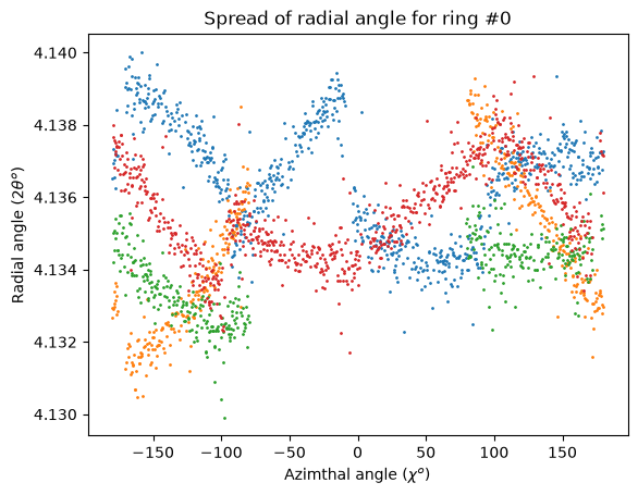
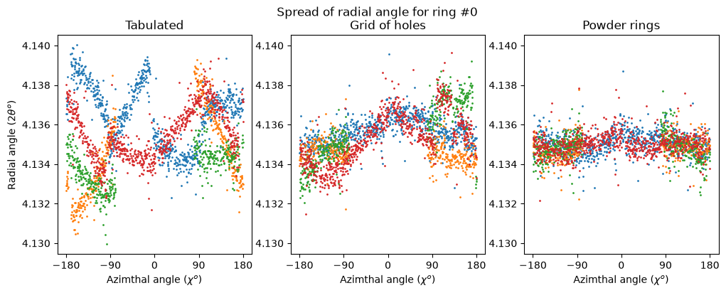
The same ring, seen through the nominal geometry of the detector, does not sit at a constant radial angle: the 2θ position of the control points of ring #0 jumps by a few millidegrees from one azimuthal sector to the next. Those steps occur at the module boundaries and are precisely what the module refinement is meant to remove — the same plot is drawn again at the end of this notebook, for the three descriptions of the detector.
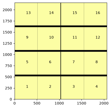
The Eiger2 4M is made of 4×4 blocks of pixels#
The detector is physically assembled from 2×4 modules, but each of them is split in two halves
by a 2-pixel gap: this gives 4×4 blocks of pixels, which are the elements whose position is
refined here. They are labelled from 1 to 16 by ndimage.label on the mask of the detector.
# This is the detector used on ID11
detector = pyFAI.detector_factory("Eiger2_CdTe_4M")
mm = MultiModuleRefinement.from_detector(detector)
ax = jupyter.display(1-detector.mask)
for i,j  in mm.modules.items():
    ax.annotate(str(i), [float(k.ravel()[0]) for k in j.center[-1::-1]])
print(mm)
MultiModule with 16 modules:
   1: Module centered at (256.0, 256.5).
   2: Module centered at (256.0, 771.5).
   3: Module centered at (256.0, 1296.5).
   4: Module centered at (256.0, 1811.5).
   5: Module centered at (806.0, 256.5).
   6: Module centered at (806.0, 771.5).
   7: Module centered at (806.0, 1296.5).
   8: Module centered at (806.0, 1811.5).
   9: Module centered at (1356.0, 256.5).
  10: Module centered at (1356.0, 771.5).
  11: Module centered at (1356.0, 1296.5).
  12: Module centered at (1356.0, 1811.5).
  13: Module centered at (1906.0, 256.5).
  14: Module centered at (1906.0, 771.5).
  15: Module centered at (1906.0, 1296.5).
  16: Module centered at (1906.0, 1811.5).
# Let all modules free, except #6 which is close to the center.

for i,j  in mm.modules.items():
    if i==6:
        mm.modules[i].fixed = True
    print(f"Module #{i:2d} {'fixed' if j.fixed else 'free'}")
Module # 1 free
Module # 2 free
Module # 3 free
Module # 4 free
Module # 5 free
Module # 6 fixed
Module # 7 free
Module # 8 free
Module # 9 free
Module #10 free
Module #11 free
Module #12 free
Module #13 free
Module #14 free
Module #15 free
Module #16 free
Calibration of the detector#
Special care must be taken to obtain sub-pixel precision:
Use a good calibrant providing thin rings ($\rm CeO_2$ 0.25µm crystalite size)
Use a monochromatic beam (55 keV)
Use a small beam (200 µm)
Use a fine capillary (500 µm) of non-absorbing material (kapton)
Rotate the capillary (360°)
Every single module of the detector should see at least one ring on each image
Several beam-center positions should be used, ideally one in the center of the detector and in the four corners
The detector should be far enough from the sample so that parallax effects are negligible
Collect very intense rings to be able to extract many control points precisely.
Control points should not be taken on the “double pixel”, so addapt the mask accordingly.
Now let us load the geometries together with their associated control points:
for i in zip(cpf, ponis):
    print(f"Loading Geometry: `{i[1]}` with control points: ", end="")
    mm.load_control_points(*i, verbose=True)
print("Number of parameters to refine (modules + configurations): ", mm.nb_param)
Loading Geometry: `geom_0001.poni` with control points: `geom_0001.npt`: CeO2 Calibrant with 769 reflections at wavelength 2.2543e-11
+------+------+
|Module|Points|
+------+------+
|     1|   869|
|     2|  1010|
|     3|   979|
|     4|   848|
|     5|   983|
|     6|   424|
|     7|   438|
|     8|   841|
|     9|   961|
|    10|   441|
|    11|   449|
|    12|   809|
|    13|   859|
|    14|   917|
|    15|   899|
|    16|   865|
+------+------+
Loading Geometry: `geom_0002.poni` with control points: `geom_0002.npt`: CeO2 Calibrant with 769 reflections at wavelength 2.2543e-11
+------+------+
|Module|Points|
+------+------+
|     1|  1565|
|     2|  1276|
|     3|   887|
|     4|   975|
|     5|  1675|
|     6|  1135|
|     7|   786|
|     8|   412|
|     9|  1630|
|    10|  1148|
|    11|   771|
|    12|   400|
|    13|  1561|
|    14|  1278|
|    15|   845|
|    16|   858|
+------+------+
Loading Geometry: `geom_0003.poni` with control points: `geom_0003.npt`: CeO2 Calibrant with 769 reflections at wavelength 2.2543e-11
+------+------+
|Module|Points|
+------+------+
|     1|  1624|
|     2|  1371|
|     3|  1350|
|     4|  1318|
|     5|  1594|
|     6|  1270|
|     7|   839|
|     8|   918|
|     9|  1605|
|    10|  1144|
|    11|   754|
|    12|   396|
|    13|  1649|
|    14|  1150|
|    15|   792|
|    16|   406|
+------+------+
Loading Geometry: `geom_0004.poni` with control points: `geom_0004.npt`: CeO2 Calibrant with 769 reflections at wavelength 2.2543e-11
+------+------+
|Module|Points|
+------+------+
|     1|  1352|
|     2|  1290|
|     3|  1293|
|     4|  1361|
|     5|   884|
|     6|   941|
|     7|   911|
|     8|   858|
|     9|   985|
|    10|   444|
|    11|   465|
|    12|   757|
|    13|   967|
|    14|   435|
|    15|   440|
|    16|   779|
+------+------+
Number of parameters to refine (modules + configurations):  65
param = mm.init_param()
print("`param` is the concatenation of the displacement of the modules (45 values) and the 4 (geometries) x 5 poni-parameters")
print(param)
print("Or in a better representation:")
mm.print_param()
`param` is the concatenation of the displacement of the modules (45 values) and the 4 (geometries) x 5 poni-parameters
[ 0.          0.          0.          0.          0.          0.
  0.          0.          0.          0.          0.          0.
  0.          0.          0.          0.          0.          0.
  0.          0.          0.          0.          0.          0.
  0.          0.          0.          0.          0.          0.
  0.          0.          0.          0.          0.          0.
  0.          0.          0.          0.          0.          0.
  0.          0.          0.          0.42051061  0.08519858  0.07923709
 -0.00045326 -0.0014653   0.42058144  0.08531912  0.14839767 -0.00229473
 -0.00143057  0.42075994  0.12025968  0.14827869 -0.00224953 -0.00138334
  0.42071487  0.11996403  0.08088361 -0.00096251 -0.00097806]
Or in a better representation:
module # 1: d0   = 0.0, d1   = 0.0, rot  = 0.0,
module # 2: d0   = 0.0, d1   = 0.0, rot  = 0.0,
module # 3: d0   = 0.0, d1   = 0.0, rot  = 0.0,
module # 4: d0   = 0.0, d1   = 0.0, rot  = 0.0,
module # 5: d0   = 0.0, d1   = 0.0, rot  = 0.0,
module # 6: Fixed
module # 7: d0   = 0.0, d1   = 0.0, rot  = 0.0,
module # 8: d0   = 0.0, d1   = 0.0, rot  = 0.0,
module # 9: d0   = 0.0, d1   = 0.0, rot  = 0.0,
module #10: d0   = 0.0, d1   = 0.0, rot  = 0.0,
module #11: d0   = 0.0, d1   = 0.0, rot  = 0.0,
module #12: d0   = 0.0, d1   = 0.0, rot  = 0.0,
module #13: d0   = 0.0, d1   = 0.0, rot  = 0.0,
module #14: d0   = 0.0, d1   = 0.0, rot  = 0.0,
module #15: d0   = 0.0, d1   = 0.0, rot  = 0.0,
module #16: d0   = 0.0, d1   = 0.0, rot  = 0.0,
geom_0001.npt: dist = 0.420511, poni1= 0.085199, poni2= 0.079237, rot1 = -0.000453, rot2 = -0.001465,
geom_0002.npt: dist = 0.420581, poni1= 0.085319, poni2= 0.148398, rot1 = -0.002295, rot2 = -0.001431,
geom_0003.npt: dist = 0.420760, poni1= 0.120260, poni2= 0.148279, rot1 = -0.002250, rot2 = -0.001383,
geom_0004.npt: dist = 0.420715, poni1= 0.119964, poni2= 0.080884, rot1 = -0.000963, rot2 = -0.000978,
mm.init_q_theo()
Both the 45 parameters describing the displacement of the modules and the 4 sets of PONI-parameters are refined at once.
%time res = mm.refine(param, method="lm")
CPU times: user 31.3 s, sys: 100 ms, total: 31.4 s
Wall time: 3.16 s
res
     message: `ftol` termination condition is satisfied.
     success: True
      status: 2
         fun: [ 4.201e-03  4.815e-03 ...  1.349e-02 -5.571e-03]
           x: [ 3.585e-01 -4.564e-01 ... -1.430e-03 -1.251e-03]
        cost: 1.7069226713085581
         jac: [[ 0.000e+00 -0.000e+00 ... -0.000e+00 -0.000e+00]
               [ 0.000e+00 -0.000e+00 ... -0.000e+00 -0.000e+00]
               ...
               [-3.676e-02 -2.445e-02 ... -1.522e+02  2.292e+02]
               [-3.736e-02 -2.353e-02 ... -1.465e+02  2.329e+02]]
        grad: [ 6.272e-07 -1.817e-06 ... -1.642e-06 -1.185e-06]
  optimality: 4.504614707911969e-06
 active_mask: [0 0 ... 0 0]
        nfev: 4
        njev: None
 chi2_before: 0.00010871623083245781
  chi2_after: 5.494150480586321e-05
     applied: True
# Precision of the fit, from the jacobian of the residuals:
sigma = mm.calc_uncertainties(res)
mm.print_param(res.x, sigma)
module # 1: d0   =  0.358486 ± 0.020636, d1   = -0.456418 ± 0.019417, rot  =  0.000954 ± 0.000028,
module # 2: d0   = -0.139337 ± 0.009246, d1   = -0.503791 ± 0.015935, rot  =  0.000844 ± 0.000026,
module # 3: d0   = -0.293870 ± 0.010414, d1   = -0.404383 ± 0.015934, rot  =  0.000216 ± 0.000026,
module # 4: d0   = -0.422150 ± 0.019388, d1   = -0.435937 ± 0.018250, rot  =  0.000323 ± 0.000028,
module # 5: d0   = -0.107558 ± 0.018163, d1   = -0.359814 ± 0.008214, rot  = -0.000020 ± 0.000027,
module # 6: Fixed
module # 7: d0   =  0.123252 ± 0.010296, d1   = -0.399504 ± 0.007484, rot  = -0.000831 ± 0.000028,
module # 8: d0   = -0.297001 ± 0.019260, d1   = -0.543292 ± 0.009200, rot  =  0.000384 ± 0.000029,
module # 9: d0   =  0.084110 ± 0.019106, d1   = -0.325008 ± 0.010226, rot  =  0.000330 ± 0.000027,
module #10: d0   = -0.057456 ± 0.010772, d1   = -0.044165 ± 0.010142, rot  =  0.000462 ± 0.000029,
module #11: d0   = -0.120670 ± 0.011741, d1   = -0.161691 ± 0.010680, rot  =  0.000591 ± 0.000029,
module #12: d0   = -0.434111 ± 0.020275, d1   = -0.144058 ± 0.011873, rot  =  0.000766 ± 0.000031,
module #13: d0   =  0.239451 ± 0.021826, d1   =  0.122557 ± 0.021241, rot  = -0.001133 ± 0.000029,
module #14: d0   = -0.097631 ± 0.011467, d1   = -0.052698 ± 0.020928, rot  =  0.000625 ± 0.000029,
module #15: d0   = -0.172935 ± 0.012377, d1   = -0.131551 ± 0.021074, rot  = -0.000168 ± 0.000030,
module #16: d0   = -0.061175 ± 0.021511, d1   =  0.086001 ± 0.022005, rot  =  0.000102 ± 0.000031,
geom_0001.npt: dist =  0.420521 ± 0.000002, poni1=  0.085221 ± 0.000014, poni2=  0.078865 ± 0.000014, rot1 = -0.001273 ± 0.000033, rot2 = -0.001533 ± 0.000032,
geom_0002.npt: dist =  0.420655 ± 0.000005, poni1=  0.085281 ± 0.000011, poni2=  0.148256 ± 0.000011, rot1 = -0.002620 ± 0.000026, rot2 = -0.001401 ± 0.000026,
geom_0003.npt: dist =  0.420832 ± 0.000005, poni1=  0.120246 ± 0.000011, poni2=  0.148148 ± 0.000011, rot1 = -0.002567 ± 0.000026, rot2 = -0.001393 ± 0.000025,
geom_0004.npt: dist =  0.420723 ± 0.000003, poni1=  0.120079 ± 0.000011, poni2=  0.080675 ± 0.000013, rot1 = -0.001430 ± 0.000029, rot2 = -0.001251 ± 0.000025,
print(f"Improvement of refined cost from {mm.cost(param)} --> {mm.cost(res.x)}")
Improvement of refined cost from 6.755191719005598 --> 3.4138453426171163
Saving the refined detector#
MultiModule.to_detector applies the displacement of every module to the corners of the
pixels of the tabulated detector and returns a Detector object where the position of the
4 corners of each pixel is stored explicitly. This is the only way to describe a detector
which is neither uniform nor contiguous, and the NeXus format is the only one able to store
it. Such a file is read back with pyFAI.detector_factory and used like any other detector,
for example in a poni-file.
# Build a detector from the displaced modules:
refined_detector = mm.to_detector()
Removing the arbitrary rigid motion#
The refinement constrains the relative position of the modules, not the position of the detector as a whole: a global translation and rotation of all the modules is exactly compensated by the poni-parameters of the four geometries. Fixing module #6 removes this singularity but leaves the whole pixel grid shifted with respect to the tabulated detector, which makes the refined values hard to interpret and the resulting poni-files hard to compare.
The Kabsch algorithm provides the rigid transformation — one rotation and one translation —
which brings the refined pixel grid as close as possible to the tabulated one, in the
least-squares sense. Applying it does not change the shape of the detector, hence neither the
quality of the calibration, it only removes the arbitrary part of the solution.
# Re-center pixels so that they are as close as possible to the tabulated detector
pixel = tabulated_detector.pixel1
pixel_coord_tab = tabulated_detector.get_pixel_corners().astype(numpy.float64)
pixel_coord_pow = refined_detector.get_pixel_corners().astype(numpy.float64)
displ_refined = numpy.sqrt(((pixel_coord_pow - pixel_coord_tab)**2).sum(axis=-1))/pixel

kabsch = Kabsch(pixel_coord_tab.reshape((-1, 3)), pixel_coord_pow.reshape((-1, 3)))
print(kabsch)
pixel_coord_cen = kabsch.correct(pixel_coord_pow.reshape((-1, 3))).reshape(pixel_coord_tab.shape)
displ_aligned = numpy.sqrt(((pixel_coord_cen - pixel_coord_tab)**2).sum(axis=-1))/pixel
Rigid transformation of angle -0.000° and translation [[ 0.00000000e+00 -1.37682783e-05 3.73835678e-05]], RMSD=0.000017
fig, ax = subplots()
ax.hist(displ_refined.ravel(), 100, label="refined before alignment", alpha=0.5)
ax.hist(displ_aligned.ravel(), 100, label="refined after alignment", alpha=0.5)
ax.set_title("Displacement of pixel corners with respect to the tabulated detector")
ax.set_xlabel("Distance in pixels")
ax.set_ylabel("Number of pixel corners")
ax.legend();
print(f"Maximum displacement, before: {displ_refined.max():.2f}, after: {displ_aligned.max():.2f}")
Maximum displacement, before: 0.92, after: 0.68
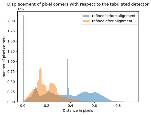
Before the alignment, the histogram shows the deformation of the detector itself, module by module: module #6 is exactly at zero since it was kept fixed during the refinement, and the other modules are spread according to how far they sit from it. After the alignment, every module has moved — module #6 included — but the mean displacement with respect to a regular pixel layout is as small as it can be. Here the rigid motion removed is almost a pure translation of half a pixel, and the maximum displacement drops from 0.92 to 0.68 pixel.
detector_file = "Eiger2CdTe_4M_ID11_powder.h5"
if os.path.exists(detector_file):
    os.remove(detector_file)
refined_detector.set_pixel_corners(pixel_coord_cen)
refined_detector.save(detector_file)
print(f"{detector_file}: {os.stat(detector_file).st_size/1e6:.1f} MB")
print(pyFAI.detector_factory(detector_file))
Eiger2CdTe_4M_ID11_powder.h5: 12.5 MB
Detector detector from NeXus file: Eiger2CdTe_4M_ID11_powder.h5 PixelSize= 75µm, 75µm BottomRight (3)
Validation of the method#
Three descriptions of the very same detector are now compared:
Tabulated: the nominal geometry of the
Eiger2 CdTe 4Mas distributed with pyFAI, where all modules are assumed to be perfectly aligned on a regular grid;Grid of holes: the geometry measured from the image of a grid-shaped mask, obtained in the Eiger2-ID11 tutorial for this very detector;
Powder rings: the geometry refined in this notebook.
Each of them is used to calibrate the 4 images, independently from each other: the very
same control points are used, the refinement starts from the same poni-files, and both the
wavelength (known from the monochromator) and rot3 are kept fixed. The residual error of
the calibration, i.e. the root mean square deviation between the measured position of the
rings and the expected one, then measures how well the detector is described: the better
the description, the smaller the residual.
def calibration_residuals(detector, fix=("wavelength", "rot3")):
    """Calibrate every image with a given detector and return the residual errors

    :param detector: the detector geometry to be validated
    :param fix: name of the parameters which are kept fixed during the refinement
    :return: list with the rms deviation to the expected ring position, in millidegree
    """
    residuals = []
    grs = {}
    for npt, poni in zip(cpf, ponis):
        cp = ControlPoints(npt)
        sg = SingleGeometry(npt, control_points=cp, calibrant=cp.calibrant,
                            detector=detector, geometry=poni)
        gr = sg.geometry_refinement
        gr.refine3(fix=list(fix))
        residuals.append(1000 * numpy.rad2deg(numpy.sqrt(gr.chi2() / gr.data.shape[0])))
        grs[os.path.basename(poni)] = gr
    return residuals, grs


grid_file = "../Eiger_Calibration/Eiger2CdTe_4M_ID11_grid.h5"  # produced by the Eiger2-ID11 tutorial
validated = {"Tabulated": pyFAI.detector_factory("Eiger2_CdTe_4M")}
if os.path.exists(grid_file):
    validated["Grid of holes"] = pyFAI.detector_factory(grid_file)
else:
    print(f"`{grid_file}` is missing: run the Eiger2-ID11 tutorial to build it")
validated["Powder rings"] = pyFAI.detector_factory(detector_file)

%time residuals = {name: calibration_residuals(det) for name, det in validated.items()}
CPU times: user 50min 22s, sys: 4.51 s, total: 50min 26s
Wall time: 57.3 s
# Residual error of the calibration, image per image:

header = [os.path.splitext(i)[0] for i in cpf]
table = ["| Detector | " + " | ".join(header) + " | Mean |",
         "|:---|" + "---:|" * (len(header) + 1)]
for name, values in residuals.items():
    table.append(f"| {name} | " + " | ".join(f"{v:.3f}" for v in values[0]) +
                 f" | **{numpy.mean(values[0]):.3f}** |")
Markdown("Residual error of the calibration, in millidegree ($2\\theta$):\n\n" + "\n".join(table))
Residual error of the calibration, in millidegree ($2\theta$):
| Detector | geom_0001 | geom_0002 | geom_0003 | geom_0004 | Mean | |:—|—:|—:|—:|—:|—:| | Tabulated | 1.808 | 2.264 | 2.424 | 1.960 | 2.114 | | Grid of holes | 1.300 | 1.886 | 2.097 | 1.404 | 1.672 | | Powder rings | 0.943 | 1.734 | 1.931 | 1.091 | 1.425 |
The three descriptions are ranked as expected: any measured geometry beats the nominal one, where the modules are assumed to be perfectly aligned on a regular grid. The powder rings even perform slightly better than the grid of holes, which is consistent with the original publication — and this without requiring any dedicated calibration object.
Visual validation of the correction#
Here we present side-by-side the spread for a single ring before and after the correction with the different detector models:
# Visualization of a ring spread
ring_idx = 0  # Ring index
fig, ax = subplots(1,3, figsize=(12,4))
for a,k in zip(ax, residuals):
    for i, gr in enumerate(residuals[k][1].values()):
        ring = numpy.array([(d[0], d[1]) for d in gr.data if d[2] == ring_idx])
        # print(len(ring))
        d0, d1 = ring.T
        tth = numpy.rad2deg(gr.tth(d0, d1))
        chi = numpy.rad2deg(gr.chi(d0, d1))
        a.scatter(chi, tth, s=1)
        a.set_title(k)
        a.set_xticks([-180, -90, 0, 90, 180])

ax[0].set_xlabel(r"Azimthal angle ($\chi ^o$)")
ax[1].set_xlabel(r"Azimthal angle ($\chi ^o$)")
ax[2].set_xlabel(r"Azimthal angle ($\chi ^o$)")
ax[0].set_ylabel(r"Radial angle (2$\theta ^o$)")
ax[1].set_ylim(ax[0].get_ylim())
ax[2].set_ylim(ax[0].get_ylim())
fig.suptitle(f"Spread of radial angle for ring #{ring_idx}");  #noqa: E703
Conclusion of the first part#
The method described by Wright et al. is now available in pyFAI, in the
pyFAI.detectors.multi_module module: the position of the 16 modules of the Eiger2 CdTe 4M
(45 parameters, one module being fixed to remove the singularity of the problem) is refined
together with the geometry of the 4 powder patterns (4 × 5 parameters), i.e. 65 parameters in
total, from the ~62000 control points extracted from the images of a $\rm CeO_2$ capillary.
The result is converted into a Detector object which holds the position of the 4 corners of
every pixel and is saved as a NeXus file: it can then be used anywhere in pyFAI, in a
poni-file, for azimuthal integration or in pyFAI-calib2.
The choice of the optimizer matters more than anything else here. With 65 parameters, a
Nelder-Mead simplex stops in a local minimum: it needs more than 3 minutes and leaves the
translations of the modules below $10^{-3}$ pixel, i.e. essentially at their initial value. A
least-squares optimizer sees the vector of residuals instead of its sum and takes advantage
of its derivatives: refine(param, method="lm") divides the cost by two in less than three
seconds, and the trf and dogbox algorithms converge towards the very same solution.
The refined module positions then become physically meaningful: with respect to a perfectly
regular pixel grid, and once the arbitrary rigid motion has been removed, the corners of the
pixels are displaced by up to 0.68 pixel, the individual modules being rotated by up to
1.13 mrad — the same order of magnitude as the values published for this very detector
(module shifts of 0.16 pixel and rotations of 0.42 mrad on average, 1.1 mrad at most).
The validation performed above measures how well the detector is described by the residual error left after calibrating each image: 2.11 m° with the tabulated detector, 1.68 m° with the grid of holes and 1.43 m° with the geometry refined here. These values are to be compared with the angle subtended by a single pixel, 10.2 m° at 42 cm: the calibration is accurate to about a seventh of a pixel, and describing the position of the modules from the powder rings gains 33% on the residual — 15% better than what the grid of holes provides, at a much lower experimental cost since no dedicated calibration object is needed.
The precision claimed in the original publication, 1/350 pixel on the module positions, is still not reached: the jacobian of the fit gives a standard deviation of 0.015 pixel on the translations and 29 µrad on the rotations, about one order of magnitude above the published values. Three directions remain open to improve this:
Quality of the control points. The peak-picking of pyFAI looks for a local maximum in two dimensions without assuming anything about the geometry. On a ring, which is sharp radially and flat azimuthally, this is an ill-posed problem. This is the subject of the second part of this notebook.
Number of the control points. The 62000 points used here are 3.6 times fewer than the 223184 peaks of the publication, where a peak is fitted along every single row and every single column of every module. This alone accounts for a factor 2 on the uncertainties.
Data collection. Only 4 beam-center positions were used. The recommendations listed at the beginning of this notebook, in particular having every module see several rings on each image, are the cheapest way to improve the conditioning of the problem.
Part 2: improving the position of the control points#
The peak-picking used in the first part makes no assumption about the geometry: it looks for a local maximum in two dimensions. On a Debye-Scherrer ring this is an ill-posed problem, since the second derivative of the signal is very different along the two directions — the peak is sharp radially and almost flat azimuthally. The tangential curvature is then dominated by the counting noise, and it leaks into the radial position through the cross-term of the Hessian, whereas only the radial position carries information about the geometry.
At this stage the geometry is approximately known, hence the radial direction is known as
well: it is the line joining the beam center, given by getFit2D, to the control point. This
second part re-extracts every control point along that line, and re-runs the very same
refinement with the improved positions. The images are needed for this, so they are
downloaded first.
import fabio
import h5py
from scipy.ndimage import map_coordinates
from silx.resources import ExternalResources

# The images, the mask of the hot pixels and the poni/npt files all come in this archive
downloader = ExternalResources("id11", "http://www.silx.org/pub/pyFAI/detector_calibration/Eiger2-ID11")
filelist = downloader.getdir("CeO2_Spatial_distortion_apr2021.tar.bz2")
images_file = [i for i in filelist if i.endswith("CeO2_Spatial_distortion_apr2021.h5")][0]
mask_file = [i for i in filelist if i.endswith("mask2.msk")][0]
hot_pixels = fabio.open(mask_file).data
print(f"images: {images_file}")
print(f"mask:   {mask_file}")
print(f"{(hot_pixels != 0).sum()} masked pixels, i.e. "
      f"{(hot_pixels != 0).sum() - (tabulated_detector.mask != 0).sum()} more than the "
      f"tabulated detector: those are the hot pixels of this very detector.")
images: /tmp/id11_testdata_kieffer/CeO2_Spatial_distortion_apr2021.tar.bz2__content/CeO2_Spatial_distortion_apr2021/CeO2_Spatial_distortion_apr2021.h5
mask:   /tmp/id11_testdata_kieffer/CeO2_Spatial_distortion_apr2021.tar.bz2__content/CeO2_Spatial_distortion_apr2021/mask2.msk
334363 masked pixels, i.e. 65843 more than the tabulated detector: those are the hot pixels of this very detector.
Radial profile of a control point#
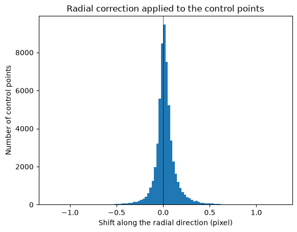
For every control point, the intensity is interpolated along the radial direction over $\pm 3.5$ pixels, i.e. a profile of 7 pixels, sampled every 0.1 pixel by bilinear interpolation. The refined radial position is the center of mass of the part of this profile which stands above a fraction of its dynamic range; the tangential coordinate is left untouched, as the data carry no information about it.
The center of mass is used rather than the position of the maximum of the profile: with a sampling of 0.1 pixel, locating a maximum from three samples measures mostly the counting noise, and doing so degrades the calibration instead of improving it. Smoothing estimators win here — for the same reason, the bilinear interpolation gives better results than a cubic spline.
A point whose profile touches a masked pixel is simply discarded: its profile is truncated, hence its center of mass is biased.
def radial_refine(image, mask, points, center, half_width=3.5, step=0.1, threshold=0.25):
    """Refine the radial position of a set of control points

    The intensity profile is interpolated along the line joining the beam center to the
    control point; the new position is the center of mass of the part of that profile which
    stands above `threshold` times its dynamic range.

    :param image: 2D array with the diffraction image
    :param mask: 2D array, non-zero where the pixel is invalid
    :param points: (N, 2) array with the (dim1, dim2) positions of the control points
    :param center: (dim1, dim2) position of the beam center, same convention
    :param half_width: half length of the profile, in pixel
    :param step: sampling of the profile, in pixel
    :param threshold: fraction of the dynamic range of the profile used as a baseline
    :return: (N, 2) refined positions, boolean array of the valid ones, radial shifts
    """
    points = numpy.ascontiguousarray(points, dtype=numpy.float64)
    delta1 = points[:, 0] - center[0]
    delta2 = points[:, 1] - center[1]
    radius = numpy.hypot(delta1, delta2)
    radius[radius == 0] = 1.0
    n1, n2 = delta1 / radius, delta2 / radius   # unit vector, pointing away from the center
    abscissa = numpy.arange(-half_width, half_width + 0.5 * step, step)
    coord1 = points[:, 0, None] + n1[:, None] * abscissa[None, :]
    coord2 = points[:, 1, None] + n2[:, None] * abscissa[None, :]
    profile = map_coordinates(image, (coord1, coord2), order=1, mode="constant", cval=0.0)
    invalid = map_coordinates(mask.astype(numpy.float32), (coord1, coord2), order=1,
                              mode="constant", cval=1.0).max(axis=1)
    baseline = profile.min(axis=1) + threshold * (profile.max(axis=1) - profile.min(axis=1))
    weight = numpy.clip(profile - baseline[:, None], 0, None)
    total = weight.sum(axis=1)
    shift = (weight * abscissa[None, :]).sum(axis=1) / numpy.where(total > 0, total, 1.0)
    valid = (total > 0) & (invalid == 0) & (abs(shift) < half_width)
    refined = points.copy()
    refined[:, 0] += numpy.where(valid, shift, 0.0) * n1
    refined[:, 1] += numpy.where(valid, shift, 0.0) * n2
    return refined, valid, shift
%%time
# Re-extract the control points of the 4 images, ring per ring
radial_dir = "radial"   # keep them apart, the `*.npt` glob at the top would pick them up
os.makedirs(radial_dir, exist_ok=True)
cpf_radial = []
all_shifts = []
with h5py.File(images_file, "r") as h5:
    for scan, (npt, poni) in enumerate(zip(cpf, ponis), start=1):
        image = h5[f"{scan}.1/instrument/eiger/data"][()].sum(axis=0).astype(numpy.float32)
        f2d = pyFAI.load(poni).getFit2D()
        # getFit2D provides the beam center with the origin at the corner of pixel (0, 0)
        center = (f2d["centerY"] - 0.5, f2d["centerX"] - 0.5)
        cp = ControlPoints(npt)
        per_ring = {}
        for d0, d1, ring in cp.getList():
            per_ring.setdefault(int(ring), []).append((d0, d1))
        new_cp = ControlPoints(calibrant=cp.calibrant)
        before = after = 0
        for ring, pts in sorted(per_ring.items()):
            refined, valid, shift = radial_refine(image, hot_pixels, numpy.array(pts), center)
            before += len(pts)
            if valid.sum():
                new_cp.append([tuple(i) for i in refined[valid]], ring=ring)
                after += valid.sum()
            all_shifts.append(shift[valid])
        dest = os.path.join(radial_dir, os.path.basename(npt))
        new_cp.save(dest)
        cpf_radial.append(dest)
        print(f"{os.path.basename(npt)}: {after}/{before} control points kept, "
              f"beam center at ({center[0]:.1f}, {center[1]:.1f})")
all_shifts = numpy.concatenate(all_shifts)
print(f"radial shift: {abs(all_shifts).mean():.3f} pixel on average, "
      f"{abs(all_shifts).max():.3f} at most")
geom_0001.npt: 11974/12592 control points kept, beam center at (1127.3, 1058.5)
geom_0002.npt: 16266/17202 control points kept, beam center at (1129.1, 1991.0)
geom_0003.npt: 17269/18180 control points kept, beam center at (1595.2, 1989.2)
geom_0004.npt: 13542/14162 control points kept, beam center at (1593.5, 1083.3)
radial shift: 0.078 pixel on average, 1.261 at most
CPU times: user 1.12 s, sys: 72.9 ms, total: 1.19 s
Wall time: 1.2 s
fig, ax = subplots()
ax.hist(all_shifts, 100)
ax.set_title("Radial correction applied to the control points")
ax.set_xlabel("Shift along the radial direction (pixel)")
ax.set_ylabel("Number of control points")
ax.axvline(0, color="black", linewidth=0.5);
Refinement of the module positions with the new control points#
The very same refinement as in the first part is performed, with the very same starting geometries: only the position of the control points has changed.
mm2 = MultiModuleRefinement.from_detector(pyFAI.detector_factory("Eiger2_CdTe_4M"))
mm2.modules[6].fixed = True
for i in zip(cpf_radial, ponis):
    mm2.load_control_points(*i, verbose=False)
print("Number of parameters to refine (modules + configurations): ", mm2.nb_param)
%time res2 = mm2.refine(method="lm")
print(f"chi2: {res2.chi2_before} --> {res2.chi2_after}  (part 1: {res.chi2_after})")
Number of parameters to refine (modules + configurations): 65
CPU times: user 31 s, sys: 75.9 ms, total: 31.1 s
Wall time: 2.99 s
chi2: 6.09614835594136e-05 --> 5.503753471311358e-06  (part 1: 5.494150480586321e-05)
# Precision of the fit, from the jacobian of the residuals:
sigma2 = mm2.calc_uncertainties(res2)
mm2.print_param(sigma=sigma2)
module # 1: d0   =  0.365987 ± 0.006717, d1   = -0.504854 ± 0.006330, rot  =  0.000980 ± 0.000009,
module # 2: d0   = -0.143981 ± 0.002998, d1   = -0.524012 ± 0.005190, rot  =  0.000841 ± 0.000009,
module # 3: d0   = -0.309345 ± 0.003378, d1   = -0.406101 ± 0.005193, rot  =  0.000234 ± 0.000009,
module # 4: d0   = -0.427335 ± 0.006309, d1   = -0.410496 ± 0.005948, rot  =  0.000254 ± 0.000009,
module # 5: d0   = -0.092247 ± 0.005912, d1   = -0.388186 ± 0.002676, rot  =  0.000022 ± 0.000009,
module # 6: Fixed
module # 7: d0   =  0.129720 ± 0.003335, d1   = -0.388888 ± 0.002430, rot  = -0.000825 ± 0.000009,
module # 8: d0   = -0.297060 ± 0.006264, d1   = -0.516881 ± 0.002990, rot  =  0.000417 ± 0.000009,
module # 9: d0   =  0.120597 ± 0.006209, d1   = -0.349385 ± 0.003323, rot  =  0.000342 ± 0.000009,
module #10: d0   = -0.030840 ± 0.003477, d1   = -0.053803 ± 0.003293, rot  =  0.000483 ± 0.000009,
module #11: d0   = -0.088193 ± 0.003801, d1   = -0.149282 ± 0.003470, rot  =  0.000576 ± 0.000010,
module #12: d0   = -0.403720 ± 0.006593, d1   = -0.103238 ± 0.003858, rot  =  0.000763 ± 0.000010,
module #13: d0   =  0.283635 ± 0.007098, d1   =  0.094936 ± 0.006913, rot  = -0.001150 ± 0.000009,
module #14: d0   = -0.034701 ± 0.003722, d1   = -0.046580 ± 0.006814, rot  =  0.000617 ± 0.000009,
module #15: d0   = -0.102044 ± 0.004026, d1   = -0.109188 ± 0.006862, rot  = -0.000109 ± 0.000010,
module #16: d0   =  0.001957 ± 0.007008, d1   =  0.115434 ± 0.007165, rot  =  0.000065 ± 0.000010,
radial/geom_0001.npt: dist =  0.420539 ± 0.000001, poni1=  0.085205 ± 0.000004, poni2=  0.078872 ± 0.000005, rot1 = -0.001257 ± 0.000011, rot2 = -0.001492 ± 0.000010,
radial/geom_0002.npt: dist =  0.420677 ± 0.000002, poni1=  0.085291 ± 0.000004, poni2=  0.148269 ± 0.000004, rot1 = -0.002596 ± 0.000009, rot2 = -0.001419 ± 0.000008,
radial/geom_0003.npt: dist =  0.420867 ± 0.000002, poni1=  0.120260 ± 0.000004, poni2=  0.148134 ± 0.000004, rot1 = -0.002612 ± 0.000008, rot2 = -0.001415 ± 0.000008,
radial/geom_0004.npt: dist =  0.420743 ± 0.000001, poni1=  0.120101 ± 0.000003, poni2=  0.080678 ± 0.000004, rot1 = -0.001423 ± 0.000009, rot2 = -0.001296 ± 0.000008,
# Same treatment as in part 1: build the detector, remove the arbitrary rigid motion, save it
refined_detector2 = mm2.to_detector()
pixel_coord_pow2 = refined_detector2.get_pixel_corners().astype(numpy.float64)
kabsch2 = Kabsch(pixel_coord_tab.reshape((-1, 3)), pixel_coord_pow2.reshape((-1, 3)))
print(kabsch2)
pixel_coord_cen2 = kabsch2.correct(pixel_coord_pow2.reshape((-1, 3))).reshape(pixel_coord_tab.shape)
displ_aligned2 = numpy.sqrt(((pixel_coord_cen2 - pixel_coord_tab)**2).sum(axis=-1))/pixel
refined_detector2.set_pixel_corners(pixel_coord_cen2)

detector_file2 = "Eiger2CdTe_4M_ID11_powder_radial.h5"
if os.path.exists(detector_file2):
    os.remove(detector_file2)
refined_detector2.save(detector_file2)
print(f"{detector_file2}: {os.stat(detector_file2).st_size/1e6:.1f} MB")
print(f"Maximum displacement of the pixel corners: {displ_aligned2.max():.2f} pixel "
      f"(part 1: {displ_aligned.max():.2f})")
Rigid transformation of angle -0.000° and translation [[ 0.00000000e+00 -1.58736839e-05 3.78180914e-05]], RMSD=0.000018
Eiger2CdTe_4M_ID11_powder_radial.h5: 12.5 MB
Maximum displacement of the pixel corners: 0.68 pixel (part 1: 0.68)
Validation#
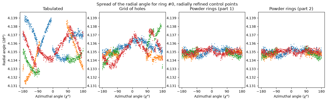
The four descriptions of the detector are now compared on the new control points: the nominal geometry, the grid of holes, and the two geometries refined from the powder rings — the one of the first part and the one obtained here. The refinement of the geometry of each image is performed exactly as before.
def calibration_residuals2(detector, cpfiles, fix=("wavelength", "rot3")):
    """Calibrate every image with a given detector and return the residual errors

    Same as `calibration_residuals`, but the control-point files are given explicitly.

    :param detector: the detector geometry to be validated
    :param cpfiles: list of files with the control points, one per geometry
    :param fix: name of the parameters which are kept fixed during the refinement
    :return: list of rms deviations to the expected ring position, in millidegree, and the
             dictionary of the refined geometries
    """
    residuals = []
    grs = {}
    for npt, poni in zip(cpfiles, ponis):
        cp = ControlPoints(npt)
        sg = SingleGeometry(npt, control_points=cp, calibrant=cp.calibrant,
                            detector=detector, geometry=poni)
        gr = sg.geometry_refinement
        gr.detector = detector  # ensure the detector is the proper one.
        gr.refine3(fix=list(fix))
        residuals.append(1000 * numpy.rad2deg(numpy.sqrt(gr.chi2() / gr.data.shape[0])))
        grs[os.path.basename(poni)] = gr
    return residuals, grs


validated2 = {"Tabulated": pyFAI.detector_factory("Eiger2_CdTe_4M")}
if os.path.exists(grid_file):
    validated2["Grid of holes"] = pyFAI.detector_factory(grid_file)
validated2["Powder rings (part 1)"] = pyFAI.detector_factory(detector_file)
validated2["Powder rings (part 2)"] = pyFAI.detector_factory(detector_file2)
%time residuals2 = {name: calibration_residuals2(det, cpf_radial) for name, det in validated2.items()}
CPU times: user 1h 46min 6s, sys: 8.2 s, total: 1h 46min 14s
Wall time: 1min 57s
# Residual error of the calibration with the radially refined control points:

header = [os.path.splitext(os.path.basename(i))[0] for i in cpf_radial]
table = ["| Detector | " + " | ".join(header) + " | Mean |",
         "|:---|" + "---:|" * (len(header) + 1)]
for name, values in residuals2.items():
    table.append(f"| {name} | " + " | ".join(f"{v:.3f}" for v in values[0]) +
                 f" | **{numpy.mean(values[0]):.3f}** |")
Markdown("Residual error of the calibration, in millidegree ($2\\theta$), "
         "using the radially refined control points:\n\n" + "\n".join(table))
Residual error of the calibration, in millidegree ($2\theta$), using the radially refined control points:
| Detector | geom_0001 | geom_0002 | geom_0003 | geom_0004 | Mean | |:—|—:|—:|—:|—:|—:| | Tabulated | 1.554 | 1.570 | 1.589 | 1.674 | 1.597 | | Grid of holes | 0.928 | 0.879 | 0.942 | 0.986 | 0.934 | | Powder rings (part 1) | 0.351 | 0.565 | 0.586 | 0.374 | 0.469 | | Powder rings (part 2) | 0.347 | 0.553 | 0.582 | 0.368 | 0.463 |
# Visualization of a ring spread, as at the end of the first part
ring_idx = 0
fig, ax = subplots(1, len(residuals2), figsize=(4*len(residuals2), 4))
for a, k in zip(ax, residuals2):
    for gr in residuals2[k][1].values():
        ring = numpy.array([(d[0], d[1]) for d in gr.data if d[2] == ring_idx])
        d0, d1 = ring.T
        a.scatter(numpy.rad2deg(gr.chi(d0, d1)), numpy.rad2deg(gr.tth(d0, d1)), s=1)
        a.set_title(k)
        a.set_xticks([-180, -90, 0, 90, 180])
        a.set_xlabel(r"Azimuthal angle ($\chi ^o$)")
ax[0].set_ylabel(r"Radial angle (2$\theta ^o$)")
for a in ax[1:]:
    a.set_ylim(ax[0].get_ylim())
fig.suptitle(f"Spread of the radial angle for ring #{ring_idx}, radially refined control points");
Conclusion#
Refining the control points along the radial direction, once the geometry is roughly known, divides the residual error of the calibration by three: from 1.43 m° at the end of the first part down to 0.46 m° here, i.e. 0.045 pixel, while the uncertainty on the position of the modules drops from 0.015 to 0.005 pixel and the one on their rotation from 29 to 9 µrad. The cost is one pass over the images, a couple of seconds, and the loss of 5% of the control points — those whose radial profile runs into a masked pixel.
Two lessons are worth keeping from this exercise:
Use the information you have. The generic peak-picking of pyFAI has to find a maximum in two dimensions because it knows nothing about the geometry. Once a first calibration is available, the radial direction is known and the problem becomes one-dimensional, which is both better posed and better conditioned. This is what the original publication does, in a different way, by fitting one peak per row and per column of every module.
Beware of estimators which do not average. The position of a maximum, obtained from a parabola through three samples, is a much noisier estimator than a center of mass over the whole profile — on this dataset it is worse than doing nothing at all.
With a standard deviation of 0.005 pixel on the module positions, the precision published for this very detector, 1/350 pixel, is now within a factor of two. The remaining gap is essentially the number of control points: 59000 here against 223184 in the publication.
Nota: this radial refinement takes advantage of the exceptional quality of this dataset — sharp rings, high dynamic range, negligible background. It is presented here as a recipe for this kind of calibration, not as a general-purpose replacement of the peak-picking of pyFAI.
print(f"Total execution time: {time.perf_counter() - start_time:.3f}s")
Total execution time: 209.784s