Distortion of Eiger2 CdTe detector from ID11#
The detector’s distortion is characterized by a Tungsten plate with a grid pattern of holes provided by Gavin Vaughan. The calibration experiment has been performed by Marie Ruat with a conventional source. Those files are not available for share, please get in contact with Marie for the experimental details.
Preprocessing#
Data were acquired with and without the grid in front of the detector. 100 frames were recorded in each case with the same exposure time. The first step is to filter out outliers using a pixel-wise median filter on the stack.
Note: a fairly recent version of FabIO is needed to read those HDF5 files produced by LImA. This notebook uses features available only in version 0.21 of pyFAI (development version for now)
%matplotlib inline
#For documentation purpose, `inline` is used to enforce the storage of the image in the notebook
# %matplotlib widget

#load many libraries ...
import time
import os
from matplotlib.pyplot import subplots
import numpy
import pyFAI
from scipy.ndimage import convolve, binary_dilation, label, distance_transform_edt
from pyFAI.ext.watershed import InverseWatershed
from pyFAI.ext.bilinear import Bilinear
from pyFAI.utils.grid import Kabsch
from scipy.spatial.distance import cdist

start_time = time.perf_counter()
print("Using pyFAI verison: ", pyFAI.version)
Using pyFAI verison: 2026.9.0
#Get the grid/flat data and filter them
!wget http://www.silx.org/pub/pyFAI/detector_calibration/Eiger2-ID11/W200um_40kVp_5mA_T4_E8_FF_noretrigger_0000.h5
!wget http://www.silx.org/pub/pyFAI/detector_calibration/Eiger2-ID11/W200um_40kVp_5mA_T4_E8_GRID_noretrigger_0000.h5
!pyFAI-average -m median W200um_40kVp_5mA_T4_E8_FF_noretrigger_0000.h5 -F numpy -o flat.npy
!pyFAI-average -m median W200um_40kVp_5mA_T4_E8_GRID_noretrigger_0000.h5 -F numpy -o grid.npy
--2026-09-15 10:01:48--  http://www.silx.org/pub/pyFAI/detector_calibration/Eiger2-ID11/W200um_40kVp_5mA_T4_E8_FF_noretrigger_0000.h5
Resolving www.silx.org (www.silx.org)... 195.154.237.27
Connecting to www.silx.org (www.silx.org)|195.154.237.27|:80... connected.
HTTP request sent, awaiting response...
200 OK
Length: 758913619 (724M)
Saving to: ‘W200um_40kVp_5mA_T4_E8_FF_noretrigger_0000.h5.18’


          W200um_40   0%[                    ]       0  --.-KB/s
W200um_40k 2%[ ] 15.09M 75.4MB/s
W200um_40kV 4%[ ] 34.56M 86.3MB/s
W200um_40kVp 7%[> ] 54.33M 90.5MB/s
W200um_40kVp_ 9%[> ] 69.67M 87.0MB/s
W200um_40kVp_5 11%[=> ] 83.54M 83.5MB/s
W200um_40kVp_5m 13%[=> ] 95.55M 79.6MB/s
W200um_40kVp_5mA 15%[==> ] 108.82M 77.7MB/s
W200um_40kVp_5mA_ 17%[==> ] 125.40M 78.3MB/s
W200um_40kVp_5mA_T 19%[==> ] 143.67M 79.8MB/s
W200um_40kVp_5mA_T4 22%[===> ] 164.93M 82.4MB/s
200um_40kVp_5mA_T4_ 25%[====> ] 187.21M 85.1MB/s
00um_40kVp_5mA_T4_E 28%[====> ] 208.43M 86.8MB/s
0um_40kVp_5mA_T4_E8 31%[=====> ] 229.76M 88.3MB/s
um_40kVp_5mA_T4_E8_ 34%[=====> ] 252.13M 90.0MB/s
m_40kVp_5mA_T4_E8_F 37%[======> ] 272.19M 90.7MB/s eta 5s
_40kVp_5mA_T4_E8_FF 40%[=======> ] 293.85M 93.1MB/s eta 5s
40kVp_5mA_T4_E8_FF_ 43%[=======> ] 316.27M 94.0MB/s eta 5s
0kVp_5mA_T4_E8_FF_n 44%[=======> ] 321.33M 87.5MB/s eta 5s
kVp_5mA_T4_E8_FF_no 45%[========> ] 327.17M 84.4MB/s eta 5s
Vp_5mA_T4_E8_FF_nor 47%[========> ] 346.99M 85.7MB/s eta 4s
p_5mA_T4_E8_FF_nore 50%[=========> ] 363.92M 86.5MB/s eta 4s
_5mA_T4_E8_FF_noret 52%[=========> ] 381.81M 89.1MB/s eta 4s
5mA_T4_E8_FF_noretr 55%[==========> ] 402.75M 90.5MB/s eta 4s
mA_T4_E8_FF_noretri 58%[==========> ] 424.51M 91.8MB/s eta 4s
A_T4_E8_FF_noretrig 61%[===========> ] 446.13M 92.3MB/s eta 3s
_T4_E8_FF_noretrigg 64%[===========> ] 467.91M 92.6MB/s eta 3s
T4_E8_FF_noretrigge 67%[============> ] 488.60M 92.6MB/s eta 3s
4_E8_FF_noretrigger 70%[=============> ] 511.05M 92.3MB/s eta 3s
_E8_FF_noretrigger_ 73%[=============> ] 532.76M 92.5MB/s eta 3s
E8_FF_noretrigger_0 76%[==============> ] 553.29M 92.5MB/s eta 2s
8_FF_noretrigger_00 79%[==============> ] 575.44M 92.4MB/s eta 2s
_FF_noretrigger_000 80%[===============> ] 582.29M 87.8MB/s eta 2s
FF_noretrigger_0000 83%[===============> ] 604.68M 88.5MB/s eta 2s
F_noretrigger_0000. 83%[===============> ] 605.89M 88.5MB/s eta 2s
_noretrigger_0000.h 86%[================> ] 627.17M 93.1MB/s eta 1s
noretrigger_0000.h5 89%[================> ] 648.42M 93.6MB/s eta 1s
oretrigger_0000.h5. 92%[=================> ] 670.61M 95.3MB/s eta 1s
retrigger_0000.h5.1 95%[==================> ] 692.25M 96.3MB/s eta 1s
etrigger_0000.h5.18 97%[==================> ] 702.61M 93.7MB/s eta 1s
W200um_40kVp_5mA_T4 100%[===================>] 723.76M  93.9MB/s    in 8.1s

2026-09-15 10:01:56 (89.8 MB/s) - ‘W200um_40kVp_5mA_T4_E8_FF_noretrigger_0000.h5.18’ saved [758913619/758913619]
--2026-09-15 10:01:56--  http://www.silx.org/pub/pyFAI/detector_calibration/Eiger2-ID11/W200um_40kVp_5mA_T4_E8_GRID_noretrigger_0000.h5
Resolving www.silx.org (www.silx.org)... 195.154.237.27
Connecting to www.silx.org (www.silx.org)|195.154.237.27|:80... connected.
HTTP request sent, awaiting response... 200 OK
Length: 484110560 (462M)
Saving to: ‘W200um_40kVp_5mA_T4_E8_GRID_noretrigger_0000.h5.18’


          W200um_40   0%[                    ]       0  --.-KB/s
W200um_40k 3%[ ] 15.15M 75.7MB/s
W200um_40kV 7%[> ] 35.02M 86.9MB/s
W200um_40kVp 12%[=> ] 57.60M 95.5MB/s
W200um_40kVp_ 16%[==> ] 78.41M 97.6MB/s
W200um_40kVp_5 20%[===> ] 93.48M 80.7MB/s
W200um_40kVp_5m 24%[===> ] 114.62M 84.4MB/s
W200um_40kVp_5mA 29%[====> ] 135.60M 87.0MB/s
W200um_40kVp_5mA_ 34%[=====> ] 157.76M 89.7MB/s
W200um_40kVp_5mA_T 38%[======> ] 179.00M 91.4MB/s
W200um_40kVp_5mA_T4 43%[=======> ] 200.54M 92.9MB/s
200um_40kVp_5mA_T4_ 48%[========> ] 222.49M 94.0MB/s
00um_40kVp_5mA_T4_E 51%[=========> ] 238.49M 92.9MB/s
0um_40kVp_5mA_T4_E8 56%[==========> ] 259.90M 93.9MB/s
um_40kVp_5mA_T4_E8_ 61%[===========> ] 281.99M 95.1MB/s
m_40kVp_5mA_T4_E8_G 65%[============> ] 302.61M 95.6MB/s eta 2s
_40kVp_5mA_T4_E8_GR 70%[=============> ] 323.58M 97.6MB/s eta 2s
40kVp_5mA_T4_E8_GRI 74%[=============> ] 345.17M 97.7MB/s eta 2s
0kVp_5mA_T4_E8_GRID 79%[==============> ] 366.32M 97.6MB/s eta 2s
kVp_5mA_T4_E8_GRID_ 83%[===============> ] 387.31M 97.9MB/s eta 2s
Vp_5mA_T4_E8_GRID_n 88%[================> ] 409.06M 97.9MB/s eta 1s
p_5mA_T4_E8_GRID_no 92%[=================> ] 427.17M 103MB/s eta 1s
_5mA_T4_E8_GRID_nor 94%[=================> ] 435.38M 98.8MB/s eta 1s
5mA_T4_E8_GRID_nore 96%[==================> ] 445.31M 94.8MB/s eta 1s
mA_T4_E8_GRID_noret 98%[==================> ] 455.17M 91.2MB/s eta 1s
W200um_40kVp_5mA_T4 100%[===================>] 461.68M  91.5MB/s    in 5.1s

2026-09-15 10:02:01 (91.3 MB/s) - ‘W200um_40kVp_5mA_T4_E8_GRID_noretrigger_0000.h5.18’ saved [484110560/484110560]
        Loading [                                        ]   0%  W200um_40kVp_5mA_T4_E8_FF_noretrigger_0000.h5


 Process median [                                        ]   0%  Feeding frames
 Process median [                                        ]   1%  Feeding frames

 Process median [                                        ]   2%  Feeding frames

 Process median [■                                       ]   3%  Feeding frames
 Process median [■                                       ]   4%  Feeding frames

 Process median [■                                       ]   5%  Feeding frames
 Process median [■■                                      ]   6%  Feeding frames

 Process median [■■                                      ]   7%  Feeding frames
 Process median [■■■                                     ]   8%  Feeding frames

 Process median [■■■                                     ]   9%  Feeding frames
 Process median [■■■                                     ]  10%  Feeding frames

 Process median [■■■■                                    ]  11%  Feeding frames
 Process median [■■■■                                    ]  12%  Feeding frames

 Process median [■■■■■                                   ]  13%  Feeding frames
 Process median [■■■■■                                   ]  14%  Feeding frames

 Process median [■■■■■                                   ]  15%  Feeding frames

 Process median [■■■■■■                                  ]  16%  Feeding frames
 Process median [■■■■■■                                  ]  17%  Feeding frames

 Process median [■■■■■■■                                 ]  18%  Feeding frames
 Process median [■■■■■■■                                 ]  19%  Feeding frames

 Process median [■■■■■■■                                 ]  20%  Feeding frames
 Process median [■■■■■■■■                                ]  21%  Feeding frames

 Process median [■■■■■■■■                                ]  22%  Feeding frames
 Process median [■■■■■■■■■                               ]  23%  Feeding frames

 Process median [■■■■■■■■■                               ]  24%  Feeding frames
 Process median [■■■■■■■■■                               ]  25%  Feeding frames

 Process median [■■■■■■■■■■                              ]  26%  Feeding frames
 Process median [■■■■■■■■■■                              ]  27%  Feeding frames

 Process median [■■■■■■■■■■■                             ]  28%  Feeding frames

 Process median [■■■■■■■■■■■                             ]  29%  Feeding frames
 Process median [■■■■■■■■■■■                             ]  30%  Feeding frames

 Process median [■■■■■■■■■■■■                            ]  31%  Feeding frames
 Process median [■■■■■■■■■■■■                            ]  32%  Feeding frames

 Process median [■■■■■■■■■■■■■                           ]  33%  Feeding frames
 Process median [■■■■■■■■■■■■■                           ]  34%  Feeding frames

 Process median [■■■■■■■■■■■■■                           ]  35%  Feeding frames
 Process median [■■■■■■■■■■■■■■                          ]  36%  Feeding frames

 Process median [■■■■■■■■■■■■■■                          ]  37%  Feeding frames
 Process median [■■■■■■■■■■■■■■■                         ]  38%  Feeding frames

 Process median [■■■■■■■■■■■■■■■                         ]  39%  Feeding frames
 Process median [■■■■■■■■■■■■■■■                         ]  40%  Feeding frames

 Process median [■■■■■■■■■■■■■■■■                        ]  41%  Feeding frames
 Process median [■■■■■■■■■■■■■■■■                        ]  42%  Feeding frames

 Process median [■■■■■■■■■■■■■■■■■                       ]  43%  Feeding frames
 Process median [■■■■■■■■■■■■■■■■■                       ]  44%  Feeding frames

 Process median [■■■■■■■■■■■■■■■■■                       ]  45%  Feeding frames

 Process median [■■■■■■■■■■■■■■■■■■                      ]  46%  Feeding frames
 Process median [■■■■■■■■■■■■■■■■■■                      ]  47%  Feeding frames

 Process median [■■■■■■■■■■■■■■■■■■■                     ]  48%  Feeding frames
 Process median [■■■■■■■■■■■■■■■■■■■                     ]  49%  Feeding frames

 Process median [■■■■■■■■■■■■■■■■■■■                     ]  50%  Feeding frames
Process median [■■■■■■■■■■■■■■■■■■■■ ] 50% Feeding frames
 Process median [■■■■■■■■■■■■■■■■■■■■                    ]  51%  Feeding frames

 Process median [■■■■■■■■■■■■■■■■■■■■                    ]  52%  Feeding frames
Process median [■■■■■■■■■■■■■■■■■■■■■ ] 53% Feeding frames
Process median [■■■■■■■■■■■■■■■■■■■■■ ] 54% Feeding frames
Process median [■■■■■■■■■■■■■■■■■■■■■■ ] 55% Feeding frames
 Process median [■■■■■■■■■■■■■■■■■■■■■■                  ]  56%  Feeding frames

 Process median [■■■■■■■■■■■■■■■■■■■■■■                  ]  57%  Feeding frames
 Process median [■■■■■■■■■■■■■■■■■■■■■■■                 ]  58%  Feeding frames

 Process median [■■■■■■■■■■■■■■■■■■■■■■■                 ]  59%  Feeding frames
 Process median [■■■■■■■■■■■■■■■■■■■■■■■■                ]  60%  Feeding frames

 Process median [■■■■■■■■■■■■■■■■■■■■■■■■                ]  61%  Feeding frames

 Process median [■■■■■■■■■■■■■■■■■■■■■■■■                ]  62%  Feeding frames
 Process median [■■■■■■■■■■■■■■■■■■■■■■■■■               ]  63%  Feeding frames

 Process median [■■■■■■■■■■■■■■■■■■■■■■■■■               ]  64%  Feeding frames
Process median [■■■■■■■■■■■■■■■■■■■■■■■■■■ ] 65% Feeding frames
Process median [■■■■■■■■■■■■■■■■■■■■■■■■■■ ] 66% Feeding frames
 Process median [■■■■■■■■■■■■■■■■■■■■■■■■■■              ]  67%  Feeding frames

 Process median [■■■■■■■■■■■■■■■■■■■■■■■■■■■             ]  68%  Feeding frames
Process median [■■■■■■■■■■■■■■■■■■■■■■■■■■■ ] 69% Feeding frames
Process median [■■■■■■■■■■■■■■■■■■■■■■■■■■■■ ] 70% Feeding frames
Process median [■■■■■■■■■■■■■■■■■■■■■■■■■■■■ ] 71% Feeding frames
Process median [■■■■■■■■■■■■■■■■■■■■■■■■■■■■ ] 72% Feeding frames
Process median [■■■■■■■■■■■■■■■■■■■■■■■■■■■■■ ] 73% Feeding frames
 Process median [■■■■■■■■■■■■■■■■■■■■■■■■■■■■■           ]  74%  Feeding frames

 Process median [■■■■■■■■■■■■■■■■■■■■■■■■■■■■■■          ]  75%  Feeding frames
Process median [■■■■■■■■■■■■■■■■■■■■■■■■■■■■■■ ] 76% Feeding frames
Process median [■■■■■■■■■■■■■■■■■■■■■■■■■■■■■■ ] 77% Feeding frames
Process median [■■■■■■■■■■■■■■■■■■■■■■■■■■■■■■■ ] 78% Feeding frames
Process median [■■■■■■■■■■■■■■■■■■■■■■■■■■■■■■■ ] 79% Feeding frames
 Process median [■■■■■■■■■■■■■■■■■■■■■■■■■■■■■■■■        ]  80%  Feeding frames

 Process median [■■■■■■■■■■■■■■■■■■■■■■■■■■■■■■■■        ]  81%  Feeding frames
Process median [■■■■■■■■■■■■■■■■■■■■■■■■■■■■■■■■ ] 82% Feeding frames
Process median [■■■■■■■■■■■■■■■■■■■■■■■■■■■■■■■■■ ] 83% Feeding frames
Process median [■■■■■■■■■■■■■■■■■■■■■■■■■■■■■■■■■ ] 84% Feeding frames
Process median [■■■■■■■■■■■■■■■■■■■■■■■■■■■■■■■■■■ ] 85% Feeding frames
Process median [■■■■■■■■■■■■■■■■■■■■■■■■■■■■■■■■■■ ] 86% Feeding frames
 Process median [■■■■■■■■■■■■■■■■■■■■■■■■■■■■■■■■■■      ]  87%  Feeding frames

 Process median [■■■■■■■■■■■■■■■■■■■■■■■■■■■■■■■■■■■     ]  88%  Feeding frames
Process median [■■■■■■■■■■■■■■■■■■■■■■■■■■■■■■■■■■■ ] 89% Feeding frames
Process median [■■■■■■■■■■■■■■■■■■■■■■■■■■■■■■■■■■■■ ] 90% Feeding frames
Process median [■■■■■■■■■■■■■■■■■■■■■■■■■■■■■■■■■■■■ ] 91% Feeding frames
Process median [■■■■■■■■■■■■■■■■■■■■■■■■■■■■■■■■■■■■ ] 92% Feeding frames
Process median [■■■■■■■■■■■■■■■■■■■■■■■■■■■■■■■■■■■■■ ] 93% Feeding frames
 Process median [■■■■■■■■■■■■■■■■■■■■■■■■■■■■■■■■■■■■■   ]  94%  Feeding frames

 Process median [■■■■■■■■■■■■■■■■■■■■■■■■■■■■■■■■■■■■■■  ]  95%  Feeding frames
Process median [■■■■■■■■■■■■■■■■■■■■■■■■■■■■■■■■■■■■■■ ] 96% Feeding frames
Process median [■■■■■■■■■■■■■■■■■■■■■■■■■■■■■■■■■■■■■■ ] 97% Feeding frames
 Process median [■■■■■■■■■■■■■■■■■■■■■■■■■■■■■■■■■■■■■■■ ]  98%  Feeding frames

 Process median [■■■■■■■■■■■■■■■■■■■■■■■■■■■■■■■■■■■■■■■ ]  99%  Computing result
Median reduction finished
        Loading [                                        ]   0%  W200um_40kVp_5mA_T4_E8_GRID_noretrigger_0000.h5


 Process median [                                        ]   0%  Feeding frames
 Process median [                                        ]   1%  Feeding frames

 Process median [                                        ]   2%  Feeding frames
Process median [■ ] 3% Feeding frames
 Process median [■                                       ]   4%  Feeding frames

 Process median [■                                       ]   5%  Feeding frames
 Process median [■■                                      ]   6%  Feeding frames

 Process median [■■                                      ]   7%  Feeding frames
Process median [■■■ ] 8% Feeding frames
 Process median [■■■                                     ]   9%  Feeding frames

 Process median [■■■                                     ]  10%  Feeding frames
 Process median [■■■■                                    ]  11%  Feeding frames

 Process median [■■■■                                    ]  12%  Feeding frames
 Process median [■■■■■                                   ]  13%  Feeding frames

 Process median [■■■■■                                   ]  14%  Feeding frames
Process median [■■■■■ ] 15% Feeding frames
 Process median [■■■■■■                                  ]  16%  Feeding frames

 Process median [■■■■■■                                  ]  17%  Feeding frames
Process median [■■■■■■■ ] 18% Feeding frames
 Process median [■■■■■■■                                 ]  19%  Feeding frames

 Process median [■■■■■■■                                 ]  20%  Feeding frames
Process median [■■■■■■■■ ] 21% Feeding frames
 Process median [■■■■■■■■                                ]  22%  Feeding frames

 Process median [■■■■■■■■■                               ]  23%  Feeding frames
Process median [■■■■■■■■■ ] 24% Feeding frames
 Process median [■■■■■■■■■                               ]  25%  Feeding frames

 Process median [■■■■■■■■■■                              ]  26%  Feeding frames
 Process median [■■■■■■■■■■                              ]  27%  Feeding frames

 Process median [■■■■■■■■■■■                             ]  28%  Feeding frames
Process median [■■■■■■■■■■■ ] 29% Feeding frames
 Process median [■■■■■■■■■■■                             ]  30%  Feeding frames

 Process median [■■■■■■■■■■■■                            ]  31%  Feeding frames
Process median [■■■■■■■■■■■■ ] 32% Feeding frames
 Process median [■■■■■■■■■■■■■                           ]  33%  Feeding frames

 Process median [■■■■■■■■■■■■■                           ]  34%  Feeding frames
Process median [■■■■■■■■■■■■■ ] 35% Feeding frames
 Process median [■■■■■■■■■■■■■■                          ]  36%  Feeding frames

 Process median [■■■■■■■■■■■■■■                          ]  37%  Feeding frames
 Process median [■■■■■■■■■■■■■■■                         ]  38%  Feeding frames

 Process median [■■■■■■■■■■■■■■■                         ]  39%  Feeding frames
Process median [■■■■■■■■■■■■■■■ ] 40% Feeding frames
 Process median [■■■■■■■■■■■■■■■■                        ]  41%  Feeding frames

 Process median [■■■■■■■■■■■■■■■■                        ]  42%  Feeding frames
 Process median [■■■■■■■■■■■■■■■■■                       ]  43%  Feeding frames

 Process median [■■■■■■■■■■■■■■■■■                       ]  44%  Feeding frames
Process median [■■■■■■■■■■■■■■■■■ ] 45% Feeding frames
Process median [■■■■■■■■■■■■■■■■■■ ] 46% Feeding frames
Process median [■■■■■■■■■■■■■■■■■■ ] 47% Feeding frames
Process median [■■■■■■■■■■■■■■■■■■■ ] 48% Feeding frames
Process median [■■■■■■■■■■■■■■■■■■■ ] 49% Feeding frames
Process median [■■■■■■■■■■■■■■■■■■■ ] 50% Feeding frames
Process median [■■■■■■■■■■■■■■■■■■■■ ] 50% Feeding frames
Process median [■■■■■■■■■■■■■■■■■■■■ ] 51% Feeding frames
Process median [■■■■■■■■■■■■■■■■■■■■ ] 52% Feeding frames
Process median [■■■■■■■■■■■■■■■■■■■■■ ] 53% Feeding frames
Process median [■■■■■■■■■■■■■■■■■■■■■ ] 54% Feeding frames
Process median [■■■■■■■■■■■■■■■■■■■■■■ ] 55% Feeding frames
Process median [■■■■■■■■■■■■■■■■■■■■■■ ] 56% Feeding frames
Process median [■■■■■■■■■■■■■■■■■■■■■■ ] 57% Feeding frames
Process median [■■■■■■■■■■■■■■■■■■■■■■■ ] 58% Feeding frames
Process median [■■■■■■■■■■■■■■■■■■■■■■■ ] 59% Feeding frames
Process median [■■■■■■■■■■■■■■■■■■■■■■■■ ] 60% Feeding frames
Process median [■■■■■■■■■■■■■■■■■■■■■■■■ ] 61% Feeding frames
Process median [■■■■■■■■■■■■■■■■■■■■■■■■ ] 62% Feeding frames
Process median [■■■■■■■■■■■■■■■■■■■■■■■■■ ] 63% Feeding frames
Process median [■■■■■■■■■■■■■■■■■■■■■■■■■ ] 64% Feeding frames
Process median [■■■■■■■■■■■■■■■■■■■■■■■■■■ ] 65% Feeding frames
Process median [■■■■■■■■■■■■■■■■■■■■■■■■■■ ] 66% Feeding frames
Process median [■■■■■■■■■■■■■■■■■■■■■■■■■■ ] 67% Feeding frames
Process median [■■■■■■■■■■■■■■■■■■■■■■■■■■■ ] 68% Feeding frames
Process median [■■■■■■■■■■■■■■■■■■■■■■■■■■■ ] 69% Feeding frames
 Process median [■■■■■■■■■■■■■■■■■■■■■■■■■■■■            ]  70%  Feeding frames

 Process median [■■■■■■■■■■■■■■■■■■■■■■■■■■■■            ]  71%  Feeding frames
Process median [■■■■■■■■■■■■■■■■■■■■■■■■■■■■ ] 72% Feeding frames
Process median [■■■■■■■■■■■■■■■■■■■■■■■■■■■■■ ] 73% Feeding frames
Process median [■■■■■■■■■■■■■■■■■■■■■■■■■■■■■ ] 74% Feeding frames
Process median [■■■■■■■■■■■■■■■■■■■■■■■■■■■■■■ ] 75% Feeding frames
Process median [■■■■■■■■■■■■■■■■■■■■■■■■■■■■■■ ] 76% Feeding frames
 Process median [■■■■■■■■■■■■■■■■■■■■■■■■■■■■■■          ]  77%  Feeding frames

 Process median [■■■■■■■■■■■■■■■■■■■■■■■■■■■■■■■         ]  78%  Feeding frames
Process median [■■■■■■■■■■■■■■■■■■■■■■■■■■■■■■■ ] 79% Feeding frames
Process median [■■■■■■■■■■■■■■■■■■■■■■■■■■■■■■■■ ] 80% Feeding frames
Process median [■■■■■■■■■■■■■■■■■■■■■■■■■■■■■■■■ ] 81% Feeding frames
Process median [■■■■■■■■■■■■■■■■■■■■■■■■■■■■■■■■ ] 82% Feeding frames
Process median [■■■■■■■■■■■■■■■■■■■■■■■■■■■■■■■■■ ] 83% Feeding frames
 Process median [■■■■■■■■■■■■■■■■■■■■■■■■■■■■■■■■■       ]  84%  Feeding frames

 Process median [■■■■■■■■■■■■■■■■■■■■■■■■■■■■■■■■■■      ]  85%  Feeding frames
Process median [■■■■■■■■■■■■■■■■■■■■■■■■■■■■■■■■■■ ] 86% Feeding frames
Process median [■■■■■■■■■■■■■■■■■■■■■■■■■■■■■■■■■■ ] 87% Feeding frames
Process median [■■■■■■■■■■■■■■■■■■■■■■■■■■■■■■■■■■■ ] 88% Feeding frames
Process median [■■■■■■■■■■■■■■■■■■■■■■■■■■■■■■■■■■■ ] 89% Feeding frames
Process median [■■■■■■■■■■■■■■■■■■■■■■■■■■■■■■■■■■■■ ] 90% Feeding frames
 Process median [■■■■■■■■■■■■■■■■■■■■■■■■■■■■■■■■■■■■    ]  91%  Feeding frames

 Process median [■■■■■■■■■■■■■■■■■■■■■■■■■■■■■■■■■■■■    ]  92%  Feeding frames
Process median [■■■■■■■■■■■■■■■■■■■■■■■■■■■■■■■■■■■■■ ] 93% Feeding frames
Process median [■■■■■■■■■■■■■■■■■■■■■■■■■■■■■■■■■■■■■ ] 94% Feeding frames
Process median [■■■■■■■■■■■■■■■■■■■■■■■■■■■■■■■■■■■■■■ ] 95% Feeding frames
Process median [■■■■■■■■■■■■■■■■■■■■■■■■■■■■■■■■■■■■■■ ] 96% Feeding frames
 Process median [■■■■■■■■■■■■■■■■■■■■■■■■■■■■■■■■■■■■■■  ]  97%  Feeding frames

 Process median [■■■■■■■■■■■■■■■■■■■■■■■■■■■■■■■■■■■■■■■ ]  98%  Feeding frames

 Process median [■■■■■■■■■■■■■■■■■■■■■■■■■■■■■■■■■■■■■■■ ]  99%  Computing result
Median reduction finished
# A couple of constants and compound dtypes ...
dt = numpy.dtype([('y', numpy.float64),
                  ('x', numpy.float64),
                  ('i', numpy.int64),
                 ])
mpl = {"cmap":"viridis",
       "interpolation":"nearest"}
flat = numpy.load("flat.npy")
grid = numpy.load("grid.npy")
fig, ax = subplots(figsize=(8,8))

ax.imshow(grid/flat, **mpl)
ax.set_title("Raw grid (normalized)");
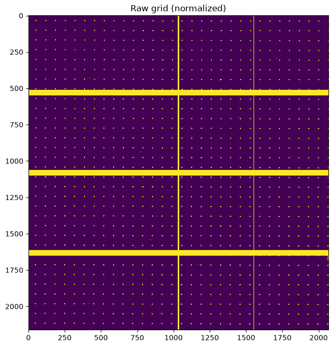
Define the right mask#
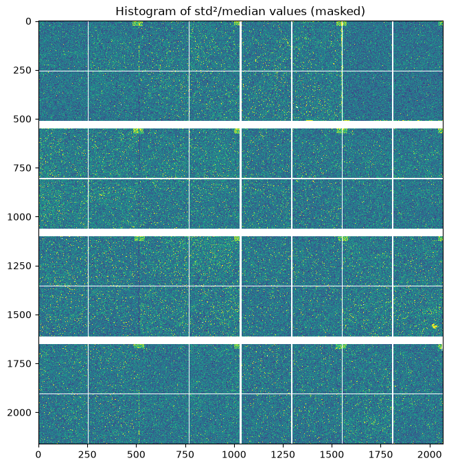
As we want to measure the position of the grid with a sub-pixel precision, it is of crucial importance to discard all pixels which have been interpolated.
The Eiger2 4M is built of 8 modules 500 kpixels, each of them consists of the assembly of 8 chips of 256x256 pixel each. Some pixels are systematically masked out as they are known to be noisy. Some pixels are also missing at the junction of the sub-modules. Finally the CdTe sensors is made of single crystals of the semi-conductor which cover 512x512 pixels. Hence one sensor covers half a module or 4 chips.
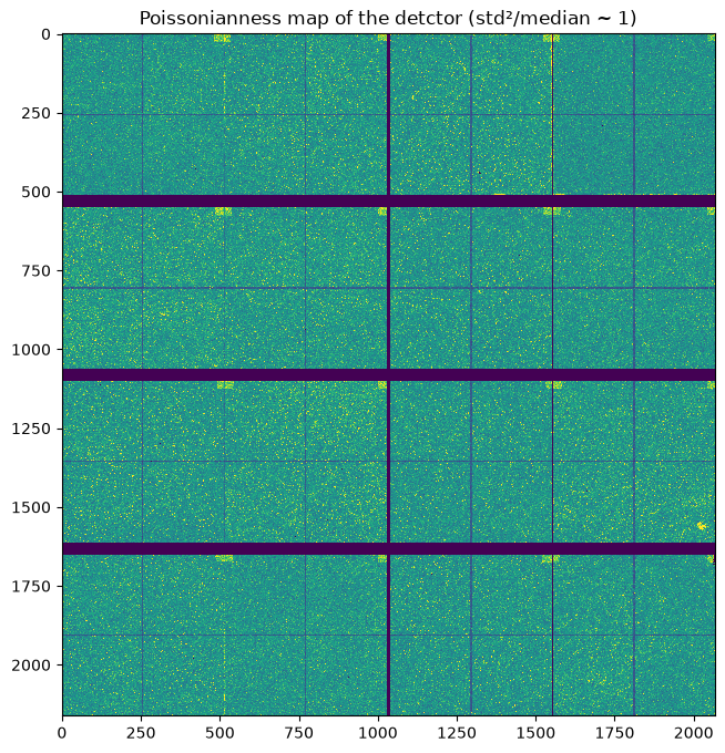
This is best demonstrated by the pixel-wise standard deviation along a stack of images like the one acquired for the flatfield.
A Poissonian detector should have a variance equal to the average signal. Thus plotting the standard deviation squared over the median highlights:
Noisy pixels which should be discarded for quantitative analysis std²>>median
Interpolated pixels which have only half/quarter of the expected noise (std²<<median).
The detector has also an internal map of invalid pixel which are set to the maximum value of the range.
!pyFAI-average -m std W200um_40kVp_5mA_T4_E8_FF_noretrigger_0000.h5 -F numpy -o flat_std.npy
        Loading [                                        ]   0%  W200um_40kVp_5mA_T4_E8_FF_noretrigger_0000.h5


    Process std [                                        ]   0%  Feeding frames
    Process std [                                        ]   1%  Feeding frames

    Process std [                                        ]   2%  Feeding frames
    Process std [■                                       ]   3%  Feeding frames

    Process std [■                                       ]   4%  Feeding frames
    Process std [■                                       ]   5%  Feeding frames

    Process std [■■                                      ]   6%  Feeding frames
    Process std [■■                                      ]   7%  Feeding frames

    Process std [■■■                                     ]   8%  Feeding frames
    Process std [■■■                                     ]   9%  Feeding frames

    Process std [■■■                                     ]  10%  Feeding frames
    Process std [■■■■                                    ]  11%  Feeding frames

    Process std [■■■■                                    ]  12%  Feeding frames
    Process std [■■■■■                                   ]  13%  Feeding frames

    Process std [■■■■■                                   ]  14%  Feeding frames
    Process std [■■■■■                                   ]  15%  Feeding frames

    Process std [■■■■■■                                  ]  16%  Feeding frames
    Process std [■■■■■■                                  ]  17%  Feeding frames

    Process std [■■■■■■■                                 ]  18%  Feeding frames
    Process std [■■■■■■■                                 ]  19%  Feeding frames

    Process std [■■■■■■■                                 ]  20%  Feeding frames
    Process std [■■■■■■■■                                ]  21%  Feeding frames

    Process std [■■■■■■■■                                ]  22%  Feeding frames
    Process std [■■■■■■■■■                               ]  23%  Feeding frames

    Process std [■■■■■■■■■                               ]  24%  Feeding frames
    Process std [■■■■■■■■■                               ]  25%  Feeding frames

    Process std [■■■■■■■■■■                              ]  26%  Feeding frames

    Process std [■■■■■■■■■■                              ]  27%  Feeding frames
    Process std [■■■■■■■■■■■                             ]  28%  Feeding frames

    Process std [■■■■■■■■■■■                             ]  29%  Feeding frames
    Process std [■■■■■■■■■■■                             ]  30%  Feeding frames

    Process std [■■■■■■■■■■■■                            ]  31%  Feeding frames
    Process std [■■■■■■■■■■■■                            ]  32%  Feeding frames

    Process std [■■■■■■■■■■■■■                           ]  33%  Feeding frames
    Process std [■■■■■■■■■■■■■                           ]  34%  Feeding frames

    Process std [■■■■■■■■■■■■■                           ]  35%  Feeding frames
    Process std [■■■■■■■■■■■■■■                          ]  36%  Feeding frames

    Process std [■■■■■■■■■■■■■■                          ]  37%  Feeding frames
    Process std [■■■■■■■■■■■■■■■                         ]  38%  Feeding frames

    Process std [■■■■■■■■■■■■■■■                         ]  39%  Feeding frames
    Process std [■■■■■■■■■■■■■■■                         ]  40%  Feeding frames

    Process std [■■■■■■■■■■■■■■■■                        ]  41%  Feeding frames
    Process std [■■■■■■■■■■■■■■■■                        ]  42%  Feeding frames

    Process std [■■■■■■■■■■■■■■■■■                       ]  43%  Feeding frames
    Process std [■■■■■■■■■■■■■■■■■                       ]  44%  Feeding frames

    Process std [■■■■■■■■■■■■■■■■■                       ]  45%  Feeding frames
    Process std [■■■■■■■■■■■■■■■■■■                      ]  46%  Feeding frames

    Process std [■■■■■■■■■■■■■■■■■■                      ]  47%  Feeding frames
    Process std [■■■■■■■■■■■■■■■■■■■                     ]  48%  Feeding frames

    Process std [■■■■■■■■■■■■■■■■■■■                     ]  49%  Feeding frames
    Process std [■■■■■■■■■■■■■■■■■■■                     ]  50%  Feeding frames

    Process std [■■■■■■■■■■■■■■■■■■■■                    ]  50%  Feeding frames
    Process std [■■■■■■■■■■■■■■■■■■■■                    ]  51%  Feeding frames

    Process std [■■■■■■■■■■■■■■■■■■■■                    ]  52%  Feeding frames
    Process std [■■■■■■■■■■■■■■■■■■■■■                   ]  53%  Feeding frames

    Process std [■■■■■■■■■■■■■■■■■■■■■                   ]  54%  Feeding frames
Process std [■■■■■■■■■■■■■■■■■■■■■■ ] 55% Feeding frames
Process std [■■■■■■■■■■■■■■■■■■■■■■ ] 56% Feeding frames
Process std [■■■■■■■■■■■■■■■■■■■■■■ ] 57% Feeding frames
    Process std [■■■■■■■■■■■■■■■■■■■■■■■                 ]  58%  Feeding frames

    Process std [■■■■■■■■■■■■■■■■■■■■■■■                 ]  59%  Feeding frames
Process std [■■■■■■■■■■■■■■■■■■■■■■■■ ] 60% Feeding frames
Process std [■■■■■■■■■■■■■■■■■■■■■■■■ ] 61% Feeding frames
Process std [■■■■■■■■■■■■■■■■■■■■■■■■ ] 62% Feeding frames
Process std [■■■■■■■■■■■■■■■■■■■■■■■■■ ] 63% Feeding frames
    Process std [■■■■■■■■■■■■■■■■■■■■■■■■■               ]  64%  Feeding frames

    Process std [■■■■■■■■■■■■■■■■■■■■■■■■■■              ]  65%  Feeding frames
Process std [■■■■■■■■■■■■■■■■■■■■■■■■■■ ] 66% Feeding frames
Process std [■■■■■■■■■■■■■■■■■■■■■■■■■■ ] 67% Feeding frames
Process std [■■■■■■■■■■■■■■■■■■■■■■■■■■■ ] 68% Feeding frames
Process std [■■■■■■■■■■■■■■■■■■■■■■■■■■■ ] 69% Feeding frames
Process std [■■■■■■■■■■■■■■■■■■■■■■■■■■■■ ] 70% Feeding frames
    Process std [■■■■■■■■■■■■■■■■■■■■■■■■■■■■            ]  71%  Feeding frames

    Process std [■■■■■■■■■■■■■■■■■■■■■■■■■■■■            ]  72%  Feeding frames
Process std [■■■■■■■■■■■■■■■■■■■■■■■■■■■■■ ] 73% Feeding frames
Process std [■■■■■■■■■■■■■■■■■■■■■■■■■■■■■ ] 74% Feeding frames
Process std [■■■■■■■■■■■■■■■■■■■■■■■■■■■■■■ ] 75% Feeding frames
Process std [■■■■■■■■■■■■■■■■■■■■■■■■■■■■■■ ] 76% Feeding frames
    Process std [■■■■■■■■■■■■■■■■■■■■■■■■■■■■■■          ]  77%  Feeding frames

    Process std [■■■■■■■■■■■■■■■■■■■■■■■■■■■■■■■         ]  78%  Feeding frames
Process std [■■■■■■■■■■■■■■■■■■■■■■■■■■■■■■■ ] 79% Feeding frames
Process std [■■■■■■■■■■■■■■■■■■■■■■■■■■■■■■■■ ] 80% Feeding frames
Process std [■■■■■■■■■■■■■■■■■■■■■■■■■■■■■■■■ ] 81% Feeding frames
Process std [■■■■■■■■■■■■■■■■■■■■■■■■■■■■■■■■ ] 82% Feeding frames
Process std [■■■■■■■■■■■■■■■■■■■■■■■■■■■■■■■■■ ] 83% Feeding frames
    Process std [■■■■■■■■■■■■■■■■■■■■■■■■■■■■■■■■■       ]  84%  Feeding frames

    Process std [■■■■■■■■■■■■■■■■■■■■■■■■■■■■■■■■■■      ]  85%  Feeding frames
Process std [■■■■■■■■■■■■■■■■■■■■■■■■■■■■■■■■■■ ] 86% Feeding frames
Process std [■■■■■■■■■■■■■■■■■■■■■■■■■■■■■■■■■■ ] 87% Feeding frames
Process std [■■■■■■■■■■■■■■■■■■■■■■■■■■■■■■■■■■■ ] 88% Feeding frames
Process std [■■■■■■■■■■■■■■■■■■■■■■■■■■■■■■■■■■■ ] 89% Feeding frames
Process std [■■■■■■■■■■■■■■■■■■■■■■■■■■■■■■■■■■■■ ] 90% Feeding frames
    Process std [■■■■■■■■■■■■■■■■■■■■■■■■■■■■■■■■■■■■    ]  91%  Feeding frames

    Process std [■■■■■■■■■■■■■■■■■■■■■■■■■■■■■■■■■■■■    ]  92%  Feeding frames
Process std [■■■■■■■■■■■■■■■■■■■■■■■■■■■■■■■■■■■■■ ] 93% Feeding frames
Process std [■■■■■■■■■■■■■■■■■■■■■■■■■■■■■■■■■■■■■ ] 94% Feeding frames
Process std [■■■■■■■■■■■■■■■■■■■■■■■■■■■■■■■■■■■■■■ ] 95% Feeding frames
Process std [■■■■■■■■■■■■■■■■■■■■■■■■■■■■■■■■■■■■■■ ] 96% Feeding frames
    Process std [■■■■■■■■■■■■■■■■■■■■■■■■■■■■■■■■■■■■■■  ]  97%  Feeding frames

    Process std [■■■■■■■■■■■■■■■■■■■■■■■■■■■■■■■■■■■■■■■ ]  98%  Feeding frames

    Process std [■■■■■■■■■■■■■■■■■■■■■■■■■■■■■■■■■■■■■■■ ]  99%  Computing result
Std reduction finished
std = numpy.load("flat_std.npy")
fig, ax = subplots(figsize=(8,8))
ax.imshow((std**2/flat).clip(0,2), **mpl)
ax.set_title("Poissonianness map of the detctor (std²/median ~ 1)");
fig, ax = subplots()
ax.hist((std**2/flat).ravel(), 100, range=(0,2))
ax.set_title("Histogram of std²/median values");
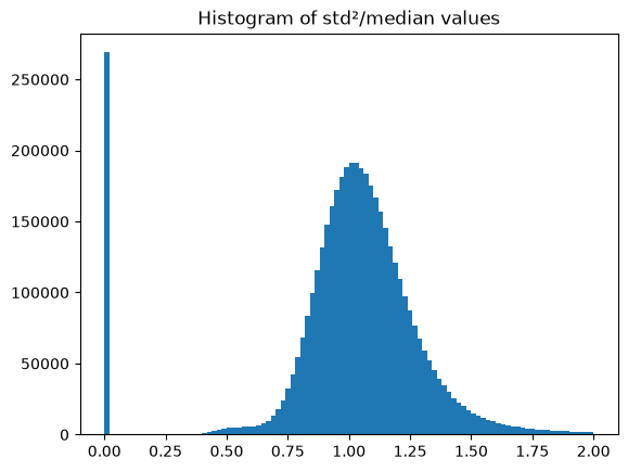
This test of Poissonian-ness is not enough to discriminate between interpolated pixels and non interpolated ones. One needs to build the mask by other methods.
# This is the default detector as definied in pyFAI according to the specification provided by Dectris:
eiger2 = pyFAI.detector_factory("Eiger2CdTe_4M")
width = eiger2.shape[1]
module_size = eiger2.MODULE_SIZE
module_gap = eiger2.MODULE_GAP
submodule_size = (256,256)
#Calculate the default mask
mask = eiger2.calc_mask()
# Mask out the interpolated pixels along X
for j in [256, 772]:
    for i in range(j, eiger2.max_shape[1],
                   eiger2.module_size[1] + eiger2.MODULE_GAP[1]):
        mask[:,i-2:i + 2] = 1
# Mask out the interpolated pixels along Y
for i in range(256, eiger2.max_shape[0],
               eiger2.module_size[0] + eiger2.MODULE_GAP[0]):
    mask[i-2:i + 2, :] = 1

# mask out the border pixels:
mask[0] = 1
mask[-1] = 1
mask[:, 0] = 1
mask[:, -1] = 1

# Finally mask out invalid/miss-behaving pixels known from the detector
mask[ flat>(flat.max()*0.99) ] = 1
pois = (std**2/flat).clip(0,2)
pois[numpy.where(mask)] = numpy.nan
fig, ax = subplots(figsize=(8,8))
ax.imshow(pois, **mpl)
ax.set_title("Histogram of std²/median values (masked)");
normalized = grid/flat
normalized[numpy.where(mask)] = numpy.nan
fig, ax = subplots(figsize=(8,8))
ax.imshow(normalized, **mpl)
ax.set_ylim(1100,1400)
ax.set_xlim(1000,1300)
ax.set_title("Zoom on one chip");
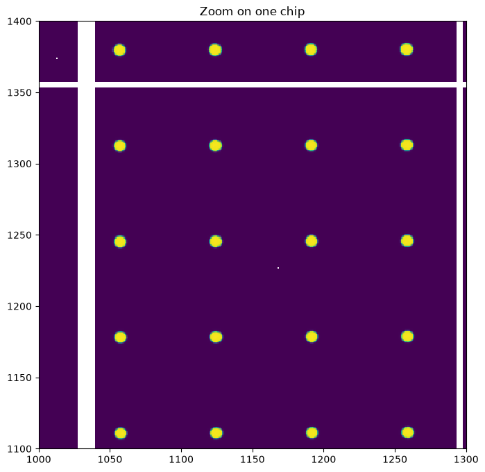
We can see we have between 8 and 16 grid spots per sub-module. This is enough as 3 are needed to localize precisely the position of the chip.
Grid spot position measurement.#
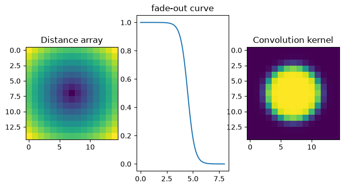
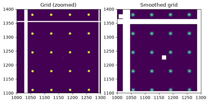
Let’s measure the position of the grid spots precisely. For this we perform a convolution with a kernel which looks like the spot itself. By zooming onto one spot, it is roughly 10 pixels wide, the kernel needs to be of odd size. The fade-out function is tuned to set precisely the spot diameter.
The masked values have been set to NaN, this ensures any spot close to a masked region get discarded automatically.
#Definition of the convolution kernel
ksize = 15
y,x = numpy.ogrid[-(ksize-1)//2:ksize//2+1,-(ksize-1)//2:ksize//2+1]
d = numpy.sqrt(y*y+x*x)

#Fade out curve definition
def fadeout(x):
    return 1/(1+numpy.exp(3*(x-4.5)))

kernel = fadeout(d)
mini=kernel.sum()
print("Integral of the kernel: ", mini)

fig,ax = subplots(1,3, figsize=(8,4))
ax[0].imshow(d)
ax[0].set_title("Distance array")

ax[1].plot(numpy.linspace(0,8,100),fadeout(numpy.linspace(0,8,100)))
ax[1].set_title("fade-out curve")

ax[2].imshow(kernel)
ax[2].set_title("Convolution kernel");
Integral of the kernel: 64.79908175810988
smooth = convolve(normalized, kernel, mode="constant", cval=0)/mini
fig,ax = subplots(1,2, figsize=(8,4))
ax[0].imshow(normalized)
ax[0].set_ylim(1100,1400)
ax[0].set_xlim(1000,1300)
ax[1].imshow(smooth)
ax[1].set_ylim(1100,1400)
ax[1].set_xlim(1000,1300)

ax[0].set_title("Grid (zoomed)")
ax[1].set_title("Smoothed grid")
pass
# Calculate a mask with all pixels close to any gap is discared
#big_mask = numpy.isnan(smooth)
big_mask = binary_dilation(numpy.isnan(smooth), iterations=ksize//2+2) #even a bit larger
#big_mask = binary_dilation(mask, iterations=ksize) #Extremely conservative !
Peak position measurement#
The center of a spot is now easily measured by segmenting out the image
iw = InverseWatershed(smooth)
iw.init()
iw.merge_singleton()
all_regions = set(iw.regions.values())

regions = [i for i in all_regions if i.size>mini]

print("Number of region segmented: {}".format(len(all_regions)))
print("Number of large enough regions : {}".format(len(regions)))
Number of region segmented: 837883
Number of large enough regions : 5968
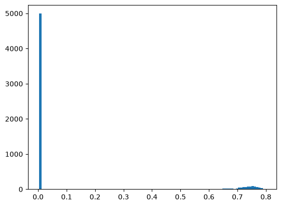
# Histogram of peak height:
s = numpy.array([i.maxi for i in regions])

fig, ax = subplots()
ax.hist(s, 100);
#Sieve-out for peak intensity
int_mini = 0.5

peaks = [(i.index//width, i.index%width) for i in regions if (i.maxi)>int_mini and
                             not big_mask[(i.index//width, i.index%width)]]
print("Number of remaining peaks with I>{}: {}".format(int_mini, len(peaks)))

peaks_raw = numpy.array(peaks)
Number of remaining peaks with I>0.5: 694
About 800 spots were found as valid out of a maximum of 1024 (64 chips with 16 spots per chip)
Those spot positions are interpolated using a second order Taylor expansion in the region around the maximum value of the smoothed image.
#Use a bilinear interpolator to localize/refine the maxima
bl = Bilinear(smooth)
ref_peaks = [bl.local_maxi(p) for p in peaks]
#Overlay raw peak coordinate and refined peak positions
fig, ax = subplots(figsize=(8,8))
ax.imshow(normalized, **mpl)
peaks_ref = numpy.array(ref_peaks)
ax.plot(peaks_raw[:,1], peaks_raw[:, 0], ".r")
ax.plot(peaks_ref[:,1],peaks_ref[:, 0], ".b")
ax.set_title("Extracted peak position (red: raw, blue: refined)")
print("Refined peak coordinate:", ref_peaks[:10], "...")
Refined peak coordinate: [(1175.3361374139786, 49.87842692434788), (642.6820283234119, 1865.566566258669), (642.8799867630005, 1932.812656134367), (643.0734554752707, 2000.0564724951982), (1175.5283335447311, 117.07293908298016), (1176.1076074764132, 318.6273694038391), (1176.3253980576992, 385.8446644693613), (1176.5270547270775, 453.0192827042192), (1176.8490638881922, 587.0088244518265), (1177.0417447797954, 654.1828182786703)] ...
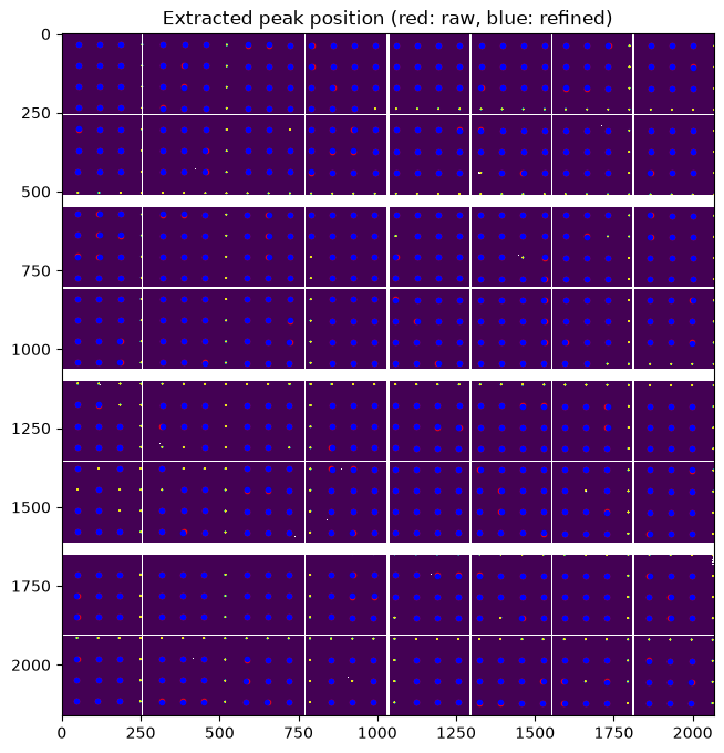
At this stage we have about 800 peaks (with sub-pixel precision) which are visually distributed on all modules and on all chips. We could have expected 16*64=1024 hence most of the spots were properly located.
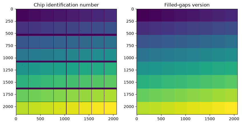
Let’s assign each peak to a module identifier. This allows to print out the number of peaks per module:
#Module identification
mid, cnt = label(numpy.isfinite(normalized), structure=numpy.ones((3,3), dtype=int))
print(cnt, "chips have been labeled")
64 chips have been labeled
# Fill the gaps in module identification array

#From http://stackoverflow.com/questions/3662361/fill-in-missing-values-with-nearest-neighbour-in-python-numpy-masked-arrays
def fill(data, invalid=None):
    """
    Replace the value of invalid 'data' cells (indicated by 'invalid')
    by the value of the nearest valid data cell

    Input:
        data:    numpy array of any dimension
        invalid: a binary array of same shape as 'data'. True cells set where data
                 value should be replaced.
                 If None (default), use: invalid  = np.isnan(data)

    Output:
        Return a filled array.
    """

    if invalid is None:
        invalid = numpy.isnan(data)

    ind = distance_transform_edt(invalid, return_distances=False, return_indices=True)
    return data[tuple(ind)]

filled_mid = fill(mid, invalid=mid==0)
fig,ax = subplots(1, 2, figsize=(10,5))
ax[0].imshow(mid, **mpl)
ax[0].set_title("Chip identification number")
ax[1].imshow(filled_mid, **mpl)
ax[1].set_title("Filled-gaps version");
yxi = numpy.array([i+(mid[round(i[0]),round(i[1])],)
                   for i in ref_peaks], dtype=dt)
print("Number of keypoint per chip:")
for i in range(1, cnt+1):
    print(f"Chip id: {i:2d} \t Number of spots: {(yxi[:]['i'] == i).sum():2d}")
Number of keypoint per chip:
Chip id:  1 	 Number of spots: 12
Chip id:  2 	 Number of spots: 12
Chip id:  3 	 Number of spots: 12
Chip id:  4 	 Number of spots: 15
Chip id:  5 	 Number of spots: 12
Chip id:  6 	 Number of spots: 12
Chip id:  7 	 Number of spots:  9
Chip id:  8 	 Number of spots:  9
Chip id:  9 	 Number of spots:  9
Chip id: 10 	 Number of spots:  9
Chip id: 11 	 Number of spots:  8
Chip id: 12 	 Number of spots: 12
Chip id: 13 	 Number of spots: 12
Chip id: 14 	 Number of spots: 11
Chip id: 15 	 Number of spots:  9
Chip id: 16 	 Number of spots:  9
Chip id: 17 	 Number of spots: 12
Chip id: 18 	 Number of spots: 12
Chip id: 19 	 Number of spots: 12
Chip id: 20 	 Number of spots: 14
Chip id: 21 	 Number of spots: 15
Chip id: 22 	 Number of spots: 15
Chip id: 23 	 Number of spots: 11
Chip id: 24 	 Number of spots: 12
Chip id: 25 	 Number of spots: 12
Chip id: 26 	 Number of spots: 12
Chip id: 27 	 Number of spots: 12
Chip id: 28 	 Number of spots: 12
Chip id: 29 	 Number of spots: 16
Chip id: 30 	 Number of spots: 16
Chip id: 31 	 Number of spots: 11
Chip id: 32 	 Number of spots:  9
Chip id: 33 	 Number of spots:  8
Chip id: 34 	 Number of spots:  7
Chip id: 35 	 Number of spots:  8
Chip id: 36 	 Number of spots:  9
Chip id: 37 	 Number of spots: 12
Chip id: 38 	 Number of spots: 12
Chip id: 39 	 Number of spots:  9
Chip id: 40 	 Number of spots:  9
Chip id: 41 	 Number of spots:  8
Chip id: 42 	 Number of spots:  9
Chip id: 43 	 Number of spots: 12
Chip id: 44 	 Number of spots: 12
Chip id: 45 	 Number of spots: 16
Chip id: 46 	 Number of spots: 16
Chip id: 47 	 Number of spots: 11
Chip id: 48 	 Number of spots: 12
Chip id: 49 	 Number of spots:  9
Chip id: 50 	 Number of spots:  9
Chip id: 51 	 Number of spots:  9
Chip id: 52 	 Number of spots:  9
Chip id: 53 	 Number of spots: 11
Chip id: 54 	 Number of spots: 11
Chip id: 55 	 Number of spots:  9
Chip id: 56 	 Number of spots:  9
Chip id: 57 	 Number of spots:  9
Chip id: 58 	 Number of spots:  9
Chip id: 59 	 Number of spots:  9
Chip id: 60 	 Number of spots:  8
Chip id: 61 	 Number of spots:  9
Chip id: 62 	 Number of spots: 12
Chip id: 63 	 Number of spots:  8
Chip id: 64 	 Number of spots:  9
Grid assignment#
The calibration is performed using a regular grid, the idea is to assign to each peak of coordinates (x,y) the integer value (X, Y) which correspond to the grid coordinate system.
The first step is to measure the grid pitch which correspond to the distance (in pixels) from one peak to the next. This is easily obtained from a pair-wise distribution function.
# pairwise distance calculation using scipy.spatial.distance.cdist

dist = cdist(peaks_ref, peaks_ref)

fig, ax = subplots()
ax.hist(dist.ravel(), 200, range=(0,200))
ax.set_title("Pair-wise distribution function")
ax.set_xlabel("Distance (pixel)")
ax.set_ylabel("Occurances");
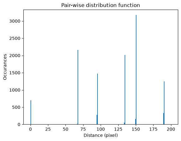
The histogram of the pair-distribution function has a first peak at 0 and the second peak between 66 and 67. The value of the step size is taken as the average of this second peak in the histogram as it corresponds to the first neighbour distance.
Two other parameters correspond to the offset, in pixels, for the grid index (X,Y) = (0,0). The easiest is to measure the smallest x and y for the first chip.
The grid looks pretty well aligned with the detector, so we will not take into account the rotation of the grid with the detector.
#from pair-wise distribution histogram
valid_pairs = dist[numpy.logical_and(60<dist, dist<70)]
step = valid_pairs.mean()
print("Average step size", step, "±", valid_pairs.std(), " pixels, condidering ", valid_pairs.size, "paires")
Average step size 67.20525103010802 ± 0.05329283719489178 pixels, condidering 2170 paires
#Refinement of the step size when considering only intra-chip distances.
intra_distances = []
inter_distances = []
extra = []
for i in range(1, cnt+1):
    locale = yxi[yxi[:]["i"] == i]
    xy = tmp = numpy.vstack((locale["x"], locale["y"])).T
    ldist = cdist(tmp, tmp).ravel()
    intra_distances.append(ldist)
    if extra:
        inter_distances.append(cdist(tmp, numpy.concatenate(extra)).ravel())
    extra.append(tmp)

valid_pairs = numpy.concatenate([ i[numpy.logical_and(60<i, i<70)] for i in intra_distances])
step = valid_pairs.mean()
print("Average step size", step, "±", valid_pairs.std(), " pixels, condidering ", valid_pairs.size, "paires")
Average step size 67.20533196766249 ± 0.03135715194578152 pixels, condidering 1888 paires
It is interesting to note the standard deviation (0.06 pixel) corresponds to the precision of our measurement, approximately 5µm. This is mostly related to the procedure for the grid manufacturing.
Any tweaking when defining the kernel prior to the convolution should be checked against this error.
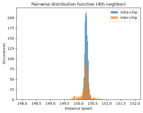
Since first neighbors are often on the same chip, so they are not representative for the distortion of the detector. Let’s rather observe the $4^{th}$ neighbor which is at 150 pixel away and corresponds to a move similar to the “knight move” at chess: 2 in one direction and one in the other. This allows not only to probe the neighboring chips in the horizontal and vertical direction but also in the diagonal. The distance for this move is $step\times\sqrt{2^2+1^2}$.
#4th neighbor: 150 pixels away
intra_pairs = numpy.concatenate([ i[numpy.logical_and(140<i, i<160)] for i in intra_distances])
inter_pairs = numpy.concatenate([ i[numpy.logical_and(140<i, i<160)] for i in inter_distances])

fig, ax = subplots()
ax.hist(intra_pairs, 200, range=(148, 152), alpha=0.7, label="intra-chip")
ax.hist(inter_pairs, 200, range=(148, 152), alpha=0.7, label="inter-chip")
ax.set_title("Pair-wise distribution function (4th neghbor)")
ax.set_xlabel("Distance (pixel)")
ax.set_ylabel("Occurances")
ax.legend()

print(f"Intra-chip average 4th neighbor distance {intra_pairs.mean():.3f}±{intra_pairs.std():.3f} pixels, condidering {intra_pairs.size} paires")
print(f"Inter-chip average 4th neighbor distance {inter_pairs.mean():.3f}±{inter_pairs.std():.3f} pixels, condidering {inter_pairs.size} paires")
Intra-chip average 4th neighbor distance 150.275±0.054 pixels, condidering 1522 paires
Inter-chip average 4th neighbor distance 150.248±0.172 pixels, condidering 904 paires
#work with the first module and fit the peak positions
first = yxi[yxi[:]["i"] == 1]
y_min = first[:]["y"].min()
x_min = first[:]["x"].min()
print("offset for the first spot: ", x_min, y_min)
offset for the first spot: 52.004524908959866 32.828430876135826
The grid looks very well aligned with the axes which makes this step easier but nothing guarantees it is perfect, so the rotation of the grid has to be measured as well. We will use Kabsch’s algorithm for this: https://en.wikipedia.org/wiki/Kabsch_algorithm
reference_1 = numpy.empty((first.size, 2))
measured_1 = numpy.empty((first.size, 2))
measured_1[:, 0] = first[:]["x"]
measured_1[:, 1] = first[:]["y"]
reference_1[:, 0] = numpy.round((first[:]["x"]-x_min)/step)*step+x_min
reference_1[:, 1] = numpy.round((first[:]["y"]-y_min)/step)*step+y_min
%time Kabsch(reference_1, measured_1)
CPU times: user 268 μs, sys: 28 μs, total: 296 μs
Wall time: 301 μs
Rigid transformation of angle -0.173° and translation [[-0.6909649 0.12761893]], RMSD=0.024761
# Print alignment info for  all chips:
kabsch_results = {}
raw_distances = []
distances = []
for i in range(1, cnt+1):
    local = yxi[yxi[:]["i"] == i]
    reference = numpy.empty((local.size, 2))
    measured = numpy.empty((local.size, 2))
    measured[:, 0] = local[:]["x"]
    measured[:, 1] = local[:]["y"]
    reference[:, 0] = numpy.round((local[:]["x"]-x_min)/step)*step+x_min
    reference[:, 1] = numpy.round((local[:]["y"]-y_min)/step)*step+y_min
    raw_distances.append(numpy.sqrt(((reference-measured)**2).sum(axis=-1)))
    res = kabsch_results[i] = Kabsch(reference, measured)
    print(f"Chip: {i:02d} \t Rmsd: {res.rmsd:.4f} \t Angle: {res.angle:.4f}°\t Displacement: {res.translation}")
    distances.append(numpy.sqrt(((reference-res.correct(measured))**2).sum(axis=-1)))
Chip: 01 	 Rmsd: 0.0248 	 Angle: -0.1730°	 Displacement: [[-0.6909649   0.12761893]]
Chip: 02 	 Rmsd: 0.0248 	 Angle: -0.1809°	 Displacement: [[-0.72426155  0.10742426]]
Chip: 03 	 Rmsd: 0.0303 	 Angle: -0.1753°	 Displacement: [[-0.62223689 -0.07963806]]
Chip: 04 	 Rmsd: 0.0337 	 Angle: -0.1768°	 Displacement: [[-0.59587368 -0.03231701]]
Chip: 05 	 Rmsd: 0.0330 	 Angle: -0.1307°	 Displacement: [[-0.20429552 -0.75913364]]
Chip: 06 	 Rmsd: 0.0561 	 Angle: -0.1277°	 Displacement: [[-0.2983904  -0.80867036]]
Chip: 07 	 Rmsd: 0.0345 	 Angle: -0.1422°	 Displacement: [[-0.41121789 -0.37125064]]
Chip: 08 	 Rmsd: 0.0641 	 Angle: -0.1457°	 Displacement: [[-0.59942082 -0.20276664]]
Chip: 09 	 Rmsd: 0.0404 	 Angle: -0.1872°	 Displacement: [[-0.76579726  0.12731278]]
Chip: 10 	 Rmsd: 0.0342 	 Angle: -0.1903°	 Displacement: [[-0.79539099  0.14046448]]
Chip: 11 	 Rmsd: 0.0413 	 Angle: -0.1881°	 Displacement: [[-0.68671072  0.04312733]]
Chip: 12 	 Rmsd: 0.0320 	 Angle: -0.1783°	 Displacement: [[-0.59199247 -0.05919715]]
Chip: 13 	 Rmsd: 0.0347 	 Angle: -0.1404°	 Displacement: [[-0.21197907 -0.64061288]]
Chip: 14 	 Rmsd: 0.0488 	 Angle: -0.1441°	 Displacement: [[-0.30332962 -0.49417302]]
Chip: 15 	 Rmsd: 0.0436 	 Angle: -0.1529°	 Displacement: [[-0.39028812 -0.17202619]]
Chip: 16 	 Rmsd: 0.0645 	 Angle: -0.1530°	 Displacement: [[-0.53952682 -0.08366957]]
Chip: 17 	 Rmsd: 0.0332 	 Angle: -0.1282°	 Displacement: [[-0.44350492 -0.45282131]]
Chip: 18 	 Rmsd: 0.0284 	 Angle: -0.1382°	 Displacement: [[-0.5336489  -0.46087496]]
Chip: 19 	 Rmsd: 0.0336 	 Angle: -0.1359°	 Displacement: [[ 0.04053861 -0.42450759]]
Chip: 20 	 Rmsd: 0.0309 	 Angle: -0.1395°	 Displacement: [[ 0.0505918  -0.37588651]]
Chip: 21 	 Rmsd: 0.0381 	 Angle: -0.0794°	 Displacement: [[ 0.59135218 -1.62307097]]
Chip: 22 	 Rmsd: 0.0384 	 Angle: -0.0831°	 Displacement: [[ 0.50085105 -1.53606914]]
Chip: 23 	 Rmsd: 0.0390 	 Angle: -0.1630°	 Displacement: [[-0.72447524  0.21841715]]
Chip: 24 	 Rmsd: 0.0598 	 Angle: -0.1639°	 Displacement: [[-0.87337121  0.30880003]]
Chip: 25 	 Rmsd: 0.0239 	 Angle: -0.1362°	 Displacement: [[-0.57824306 -0.4258471 ]]
Chip: 26 	 Rmsd: 0.0276 	 Angle: -0.1357°	 Displacement: [[-0.50886814 -0.4420399 ]]
Chip: 27 	 Rmsd: 0.0326 	 Angle: -0.1417°	 Displacement: [[-0.04346238 -0.34708051]]
Chip: 28 	 Rmsd: 0.0255 	 Angle: -0.1454°	 Displacement: [[-0.02127574 -0.26708116]]
Chip: 29 	 Rmsd: 0.0237 	 Angle: -0.0869°	 Displacement: [[ 0.49668335 -1.49343537]]
Chip: 30 	 Rmsd: 0.0316 	 Angle: -0.0861°	 Displacement: [[ 0.49394606 -1.49039259]]
Chip: 31 	 Rmsd: 0.0282 	 Angle: -0.1650°	 Displacement: [[-0.73415799  0.22278325]]
Chip: 32 	 Rmsd: 0.0296 	 Angle: -0.1616°	 Displacement: [[-0.82625185  0.1690789 ]]
Chip: 33 	 Rmsd: 0.0384 	 Angle: -0.1597°	 Displacement: [[-1.15541469  0.16513495]]
Chip: 34 	 Rmsd: 0.0310 	 Angle: -0.1642°	 Displacement: [[-1.16143042  0.13333022]]
Chip: 35 	 Rmsd: 0.0340 	 Angle: -0.1647°	 Displacement: [[-0.71671318  0.18619975]]
Chip: 36 	 Rmsd: 0.0294 	 Angle: -0.1755°	 Displacement: [[-0.85033103  0.29314307]]
Chip: 37 	 Rmsd: 0.0277 	 Angle: -0.1765°	 Displacement: [[-0.82510278  0.5371125 ]]
Chip: 38 	 Rmsd: 0.0257 	 Angle: -0.1764°	 Displacement: [[-0.82625902  0.54001968]]
Chip: 39 	 Rmsd: 0.0195 	 Angle: -0.1812°	 Displacement: [[-0.89522352  0.67356253]]
Chip: 40 	 Rmsd: 0.0329 	 Angle: -0.1901°	 Displacement: [[-1.23105807  0.98025776]]
Chip: 41 	 Rmsd: 0.0460 	 Angle: -0.1556°	 Displacement: [[-1.04670008  0.25925841]]
Chip: 42 	 Rmsd: 0.0449 	 Angle: -0.1612°	 Displacement: [[-1.09221711  0.22087856]]
Chip: 43 	 Rmsd: 0.0636 	 Angle: -0.1706°	 Displacement: [[-0.8312005  0.3216271]]
Chip: 44 	 Rmsd: 0.0537 	 Angle: -0.1701°	 Displacement: [[-0.71343017  0.27793948]]
Chip: 45 	 Rmsd: 0.0449 	 Angle: -0.1781°	 Displacement: [[-0.85541633  0.61921632]]
Chip: 46 	 Rmsd: 0.0402 	 Angle: -0.1864°	 Displacement: [[-1.06137394  0.81638021]]
Chip: 47 	 Rmsd: 0.0360 	 Angle: -0.1984°	 Displacement: [[-1.27510012  1.19609682]]
Chip: 48 	 Rmsd: 0.0395 	 Angle: -0.2014°	 Displacement: [[-1.47410042  1.33135928]]
Chip: 49 	 Rmsd: 0.0266 	 Angle: -0.0881°	 Displacement: [[1.50707147 0.26287883]]
Chip: 50 	 Rmsd: 0.0377 	 Angle: -0.0921°	 Displacement: [[1.48264943 0.25954151]]
Chip: 51 	 Rmsd: 0.0400 	 Angle: -0.1923°	 Displacement: [[-1.77935992  0.79494073]]
Chip: 52 	 Rmsd: 0.0311 	 Angle: -0.1969°	 Displacement: [[-1.78838175  0.84336987]]
Chip: 53 	 Rmsd: 0.0239 	 Angle: -0.1119°	 Displacement: [[ 1.00654489 -0.92414206]]
Chip: 54 	 Rmsd: 0.0255 	 Angle: -0.1088°	 Displacement: [[ 1.13511599 -1.00440956]]
Chip: 55 	 Rmsd: 0.0272 	 Angle: -0.1904°	 Displacement: [[-1.54792583  1.38993539]]
Chip: 56 	 Rmsd: 0.0389 	 Angle: -0.1945°	 Displacement: [[-1.72947961  1.57954715]]
Chip: 57 	 Rmsd: 0.0496 	 Angle: -0.0838°	 Displacement: [[1.61838646 0.3969453 ]]
Chip: 58 	 Rmsd: 0.0377 	 Angle: -0.0913°	 Displacement: [[1.48047925 0.39224844]]
Chip: 59 	 Rmsd: 0.0423 	 Angle: -0.2061°	 Displacement: [[-2.28458243  1.08288572]]
Chip: 60 	 Rmsd: 0.0294 	 Angle: -0.2061°	 Displacement: [[-2.15062133  1.14197447]]
Chip: 61 	 Rmsd: 0.0195 	 Angle: -0.1183°	 Displacement: [[ 0.75853959 -0.66529868]]
Chip: 62 	 Rmsd: 0.0326 	 Angle: -0.1096°	 Displacement: [[ 1.12784628 -0.83149603]]
Chip: 63 	 Rmsd: 0.0238 	 Angle: -0.1922°	 Displacement: [[-1.62038317  1.61374901]]
Chip: 64 	 Rmsd: 0.0400 	 Angle: -0.1973°	 Displacement: [[-1.80160201  1.8169484 ]]
ndistances = numpy.concatenate(distances)
nraw_distances = numpy.concatenate(raw_distances)

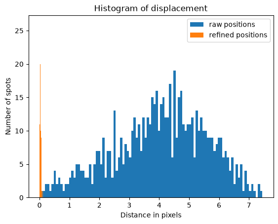
fig, ax = subplots()
ax.hist(nraw_distances, bins=100, label="raw positions")
ax.hist(ndistances, bins=100, label="refined positions")
ax.set_title("Histogram of displacement")
ax.set_xlabel("Distance in pixels")
ax.set_ylabel("Number of spots")
ax.legend();
Reconstruction of the pixel position#
The pixel position can be obtained from the standard Pilatus detector. Each module is then displaced according to the fitted values.
%%time
pixel_coord = pyFAI.detector_factory("Eiger2CdTe_4M").get_pixel_corners().astype(numpy.float64)
pixel_coord_raw = pixel_coord.copy()

for module in range(1, cnt+1):
    # Extract the pixel corners for one module
    module_idx = numpy.where(filled_mid  == module)
    one_module = pixel_coord_raw[module_idx]


    #retrieve the fitted values
    res = kabsch_results[module]

    #z = one_module[...,0]
    y = one_module[...,1].ravel()/eiger2.pixel1
    x = one_module[...,2].ravel()/eiger2.pixel2
    xy_initial = numpy.vstack((x, y)).T
    xy_aligned = res.correct(xy_initial)

    one_module[...,1] = (xy_aligned[:,1] * eiger2.pixel1).reshape(one_module.shape[:-1])
    one_module[...,2] = (xy_aligned[:,0] * eiger2.pixel2).reshape(one_module.shape[:-1])
    #Update the array
    pixel_coord[module_idx] = one_module
CPU times: user 7.95 s, sys: 133 ms, total: 8.08 s
Wall time: 1.6 s
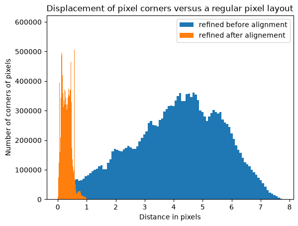
# displacement for every pixel corner (before/after global displacement):
displ_refined = numpy.sqrt(((pixel_coord - pixel_coord_raw)**2).sum(axis=-1))/eiger2.pixel1

global_ref = Kabsch(pixel_coord_raw.reshape((-1, 3)), pixel_coord.reshape((-1, 3)))
new_pixel_coord = global_ref.correct(pixel_coord.reshape((-1, 3))).reshape(pixel_coord_raw.shape)
displ_aligned = numpy.sqrt(((new_pixel_coord - pixel_coord_raw)**2).sum(axis=-1))/eiger2.pixel1
fig, ax = subplots()
ax.hist(displ_refined.ravel(), 100, label="refined before alignment")
ax.hist(displ_aligned.ravel(), 100, label="refined after alignement")
ax.set_title("Displacement of pixel corners versus a regular pixel layout")
ax.set_xlabel("Distance in pixels")
ax.set_ylabel("Number of corners of pixels")
ax.legend();
Validation of the distortion#
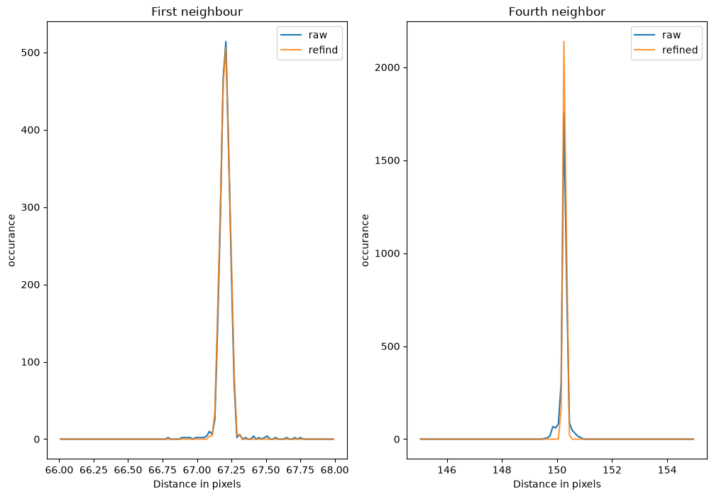
To validate the new pixel layout, we can use the new grid to calculate the spot position in space and look how well aligned they are.
First we build a function which performs the bilinear interpolation of any detector coordinate (return a 3D position). This function is then used to calculate the position for the original grid and for the corrected grid.
As previously, all spot distances are calculated and histogrammed. The standard deviation is used to evaluate how much was gained.
def intepolate_3d(yx, coord=pixel_coord_raw):
    y,x = yx
    X = int(x)
    Y = int(y)
    pixel =  coord[Y,X]
    #print(pixel)
    dx = x - X
    dy = y - Y
    res = pixel[0]*(1.0-dx)*(1.0-dy)+\
          pixel[3]*dx*(1.0-dy)+\
          pixel[1]*(1.0-dx)*dy+\
          pixel[2]*dx*dy
    return res
intepolate_3d((0.99,0.01))
array([0.00000000e+00, 7.42500035e-05, 7.50000036e-07])
raw_pixel_64 = pixel_coord_raw.astype("float64")/eiger2.pixel1
new_pixel_64 = new_pixel_coord.astype("float64")/eiger2.pixel1

spot3d_raw = numpy.array([intepolate_3d(i, coord=raw_pixel_64) for i in ref_peaks])
spot3d_ref = numpy.array([intepolate_3d(i, coord=new_pixel_64) for i in ref_peaks])

dist_raw = cdist(spot3d_raw, spot3d_raw)
valid_raw = dist_raw[numpy.logical_and(65<dist_raw, dist_raw<70)]

dist_ref = cdist(spot3d_ref, spot3d_ref)
valid_ref = dist_ref[numpy.logical_and(65<dist_ref, dist_ref<70)]
fig,ax = subplots(1, 2, figsize=(12,8))
valid1_raw = dist_raw[numpy.logical_and(65<dist_raw, dist_raw<70)]
valid1_ref = dist_ref[numpy.logical_and(65<dist_ref, dist_ref<70)]
h1_raw = numpy.histogram(valid1_raw, 100, range=(66, 68))
h1_ref = numpy.histogram(valid1_ref, 100, range=(66, 68))
x = 0.5*(h1_raw[1][1:]+h1_raw[1][:-1])
ax[0].plot(x, h1_raw[0], label="raw")
ax[0].plot(x, h1_ref[0], label="refind", alpha=0.8)
ax[0].legend()
ax[0].set_title("First neighbour")
ax[0].set_xlabel("Distance in pixels")
ax[0].set_ylabel("occurance")

valid2_raw = dist_raw[numpy.logical_and(145<dist_raw, dist_raw<155)]
valid2_ref = dist_ref[numpy.logical_and(145<dist_ref, dist_ref<155)]
h2_raw = numpy.histogram(valid2_raw, 100, range=(145, 155))
h2_ref = numpy.histogram(valid2_ref, 100, range=(145, 155))
x = 0.5*(h2_raw[1][1:]+h2_raw[1][:-1])
ax[1].plot(x, h2_raw[0], label="raw")
ax[1].plot(x, h2_ref[0], label="refined", alpha=0.8)
ax[1].legend()
ax[1].set_title("Fourth neighbor")
ax[1].set_xlabel("Distance in pixels")
ax[1].set_ylabel("occurance")
print("Distance of  first neighbor before: "+f"{valid1_raw.mean():.4f} ± {valid1_raw.std():.4f} after: {valid1_ref.mean():.4f} ± {valid1_ref.std():.4f}")
print("Distance of fourth neighbor before: "+f"{valid2_raw.mean():.4f} ± {valid2_raw.std():.4f} after: {valid2_ref.mean():.4f} ± {valid2_ref.std():.4f}")
Distance of  first neighbor before: 67.2053 ± 0.0533 after: 67.2046 ± 0.0328
Distance of fourth neighbor before: 150.2604 ± 0.1324 after: 150.2764 ± 0.0470
#Saving of the result as a distortion file usable in pyFAI
dest = "Eiger2CdTe_4M_ID11_grid.h5"
if os.path.exists(dest):
    os.unlink(dest)
eiger2.set_pixel_corners(new_pixel_coord.astype(numpy.float32))
eiger2.mask = eiger2.calc_mask() + flat>(flat.max()*0.9)
eiger2.save(dest)
Conclusion#
The distortion measured on the Eiger2 CdTe 4M detector for ID11 are small (<1 pixel, 75µm) but measurable and can be corrected to precision of 5µm using the displacement matrix.
print(f"Total execution time: {time.perf_counter()-start_time:.3f}s")
Total execution time: 66.546s